Count and Rate Outcomes: Rate Ratio Analysis

Overview

This vignette demonstrates how to use ML-UMR for count/rate outcomes where the treatment effect is measured as a rate ratio (RR). Common applications include:

Exacerbation rates in COPD/asthma
Relapse rates in multiple sclerosis
Infection rates (e.g., UTIs, respiratory infections)
Adverse event rates
Hospitalization rates
Fracture rates in osteoporosis

The Poisson likelihood models event counts accounting for varying exposure times (follow-up duration).

Clinical Scenario

Consider comparing two treatments for chronic obstructive pulmonary disease (COPD):

Treatment A (index): New inhaled therapy - IPD available from a Phase 3 trial
Treatment B (comparator): Standard inhaled corticosteroid - Only published aggregate data available

The primary endpoint is the annualized rate of moderate-to-severe COPD exacerbations.

library(mlumr)
library(dplyr)
library(ggplot2)

Step 1: Prepare the Data

Understanding Rate Data

For Poisson models, we need: - Event count: Number of events per patient - Exposure time: Follow-up time (person-years at risk)

The rate = events / exposure time.

Simulate Realistic Clinical Trial Data

set.seed(2024)

# --- Index Treatment (IPD) ---
n_index <- 300

# Patient characteristics
ipd_data <- data.frame(
  patient_id = 1:n_index,
  treatment = "Treatment_A",

  # Baseline characteristics (prognostic factors)
  age = rnorm(n_index, mean = 65, sd = 8),
  fev1_percent = rnorm(n_index, mean = 45, sd = 12),  # % predicted FEV1
  prior_exacerbations = rpois(n_index, lambda = 1.5), # Prior year count
  smoker = rbinom(n_index, 1, prob = 0.35)            # Current smoker
)

# Follow-up time varies (mean ~1 year)
ipd_data$followup_years <- rgamma(n_index, shape = 10, rate = 10)

# True model parameters for Treatment A (log-rate scale)
alpha_A <- log(0.8)  # Baseline rate ~0.8 events/year
beta_age <- 0.02     # Older = higher rate
beta_fev1 <- -0.015  # Lower FEV1 = higher rate
beta_prior <- 0.3    # Prior exacerbations strongly predictive
beta_smoker <- 0.25  # Smoking increases rate

# Generate event counts
log_rate_A <- with(ipd_data, {
  alpha_A +
    beta_age * (age - 65) +
    beta_fev1 * (fev1_percent - 45) +
    beta_prior * (prior_exacerbations - 1.5) +
    beta_smoker * smoker
})

ipd_data$exacerbation_count <- rpois(n_index,
  lambda = exp(log_rate_A) * ipd_data$followup_years)

# --- Comparator Treatment (AgD) ---
# Different population (older, more severe disease)
n_comparator <- 250

# True parameters for Treatment B (less effective)
alpha_B <- log(1.1)  # Higher baseline rate

# Simulate comparator population (not observed)
age_comp <- rnorm(n_comparator, mean = 68, sd = 7)
fev1_comp <- rnorm(n_comparator, mean = 40, sd = 10)
prior_comp <- rpois(n_comparator, lambda = 2.0)
smoker_comp <- rbinom(n_comparator, 1, prob = 0.30)
followup_comp <- rgamma(n_comparator, shape = 10, rate = 10)

log_rate_B <- alpha_B +
  beta_age * (age_comp - 65) +
  beta_fev1 * (fev1_comp - 45) +
  beta_prior * (prior_comp - 1.5) +
  beta_smoker * smoker_comp

events_comp <- rpois(n_comparator, lambda = exp(log_rate_B) * followup_comp)

# Create aggregate summary (what's published)
agd_data <- data.frame(
  study = "Comparator_Study",
  treatment = "Treatment_B",

  # Outcome summary
  total_events = sum(events_comp),
  total_exposure = sum(followup_comp),

  # Covariate summaries
  age_mean = mean(age_comp),
  age_sd = sd(age_comp),
  fev1_percent_mean = mean(fev1_comp),
  fev1_percent_sd = sd(fev1_comp),
  prior_exacerbations_mean = mean(prior_comp),
  prior_exacerbations_sd = sd(prior_comp),
  smoker_mean = mean(smoker_comp)  # Proportion (binary)
)

# Display summary
cat("IPD Summary (Treatment A):\n")
#> IPD Summary (Treatment A):
cat("  N =", n_index, "\n")
#>   N = 300
cat("  Total events =", sum(ipd_data$exacerbation_count), "\n")
#>   Total events = 294
cat("  Total exposure =", round(sum(ipd_data$followup_years), 1), "person-years\n")
#>   Total exposure = 300 person-years
cat("  Crude rate =", round(sum(ipd_data$exacerbation_count) /
    sum(ipd_data$followup_years), 2), "events/year\n")
#>   Crude rate = 0.98 events/year
cat("  Age (mean/SD):", round(mean(ipd_data$age), 1), "/",
    round(sd(ipd_data$age), 1), "\n")
#>   Age (mean/SD): 65.3 / 7.9
cat("  FEV1% (mean/SD):", round(mean(ipd_data$fev1_percent), 1), "/",
    round(sd(ipd_data$fev1_percent), 1), "\n")
#>   FEV1% (mean/SD): 45.1 / 11.7
cat("  Prior exacerbations (mean):", round(mean(ipd_data$prior_exacerbations), 2), "\n")
#>   Prior exacerbations (mean): 1.37
cat("  Current smokers:", round(mean(ipd_data$smoker) * 100, 1), "%\n\n")
#>   Current smokers: 36.7 %

cat("AgD Summary (Treatment B):\n")
#> AgD Summary (Treatment B):
cat("  N =", n_comparator, "\n")
#>   N = 250
cat("  Total events =", agd_data$total_events, "\n")
#>   Total events = 445
cat("  Total exposure =", round(agd_data$total_exposure, 1), "person-years\n")
#>   Total exposure = 248.2 person-years
cat("  Crude rate =", round(agd_data$total_events / agd_data$total_exposure, 2),
    "events/year\n")
#>   Crude rate = 1.79 events/year
cat("  Age (mean/SD):", round(agd_data$age_mean, 1), "/",
    round(agd_data$age_sd, 1), "\n")
#>   Age (mean/SD): 68.1 / 6.5
cat("  FEV1% (mean/SD):", round(agd_data$fev1_percent_mean, 1), "/",
    round(agd_data$fev1_percent_sd, 1), "\n")
#>   FEV1% (mean/SD): 39.7 / 9.7
cat("  Prior exacerbations (mean):", round(agd_data$prior_exacerbations_mean, 2), "\n")
#>   Prior exacerbations (mean): 2.03
cat("  Current smokers:", round(agd_data$smoker_mean * 100, 1), "%\n")
#>   Current smokers: 30.8 %

Key Population Differences

cat("\nPopulation Differences (Index - Comparator):\n")
#> 
#> Population Differences (Index - Comparator):
cat("  Age:", round(mean(ipd_data$age) - agd_data$age_mean, 1), "years\n")
#>   Age: -2.7 years
cat("  FEV1%:", round(mean(ipd_data$fev1_percent) - agd_data$fev1_percent_mean, 1), "%\n")
#>   FEV1%: 5.4 %
cat("  Prior exacerbations:",
    round(mean(ipd_data$prior_exacerbations) - agd_data$prior_exacerbations_mean, 2), "\n")
#>   Prior exacerbations: -0.66
cat("  Current smokers:",
    round((mean(ipd_data$smoker) - agd_data$smoker_mean) * 100, 1), "percentage points\n")
#>   Current smokers: 5.9 percentage points

cat("\nThe comparator population is older with more severe disease.\n")
#> 
#> The comparator population is older with more severe disease.
cat("A naive comparison would be confounded by these differences.\n")
#> A naive comparison would be confounded by these differences.

Step 2: Set Up ML-UMR Data Structures

Prepare IPD

ipd <- set_ipd_unanchored(
  data = ipd_data,
  treatment = "treatment",
  outcome = "exacerbation_count",
  covariates = c("age", "fev1_percent", "prior_exacerbations", "smoker"),
  likelihood = "poisson",
  E = "followup_years"  # Exposure time column
)

print(ipd)
#> $data
#> # A tibble: 300 × 8
#>    .study    .trt   .outcome    .E   age fev1_percent prior_exacerbations smoker
#>    <chr>     <chr>     <int> <dbl> <dbl>        <dbl>               <int>  <int>
#>  1 IPD_Study Treat…        0 1.10   72.9         53.5                   0      0
#>  2 IPD_Study Treat…        1 0.776  68.7         37.4                   0      0
#>  3 IPD_Study Treat…        1 0.782  64.1         41.2                   3      1
#>  4 IPD_Study Treat…        3 1.28   63.3         57.8                   2      0
#>  5 IPD_Study Treat…        1 0.950  74.3         64.1                   2      1
#>  6 IPD_Study Treat…        2 0.757  75.3         50.4                   3      1
#>  7 IPD_Study Treat…        1 0.835  69.3         43.7                   1      0
#>  8 IPD_Study Treat…        0 1.63   64.0         53.6                   2      0
#>  9 IPD_Study Treat…        1 0.924  55.2         47.2                   2      1
#> 10 IPD_Study Treat…        2 1.03   56.0         60.8                   4      1
#> # ℹ 290 more rows
#> 
#> $n
#> [1] 300
#> 
#> $n_events
#> [1] 294
#> 
#> $treatment
#> [1] "Treatment_A"
#> 
#> $covariates
#> [1] "age"                 "fev1_percent"        "prior_exacerbations"
#> [4] "smoker"             
#> 
#> $likelihood
#> [1] "poisson"
#> 
#> $type
#> [1] "ipd"
#> 
#> attr(,"class")
#> [1] "ipd_unanchored" "list"

Prepare AgD

For Poisson likelihood AgD, we need: - outcome_r: Total event count - outcome_E: Total exposure (person-years)

agd <- set_agd_unanchored(
  data = agd_data,
  treatment = "treatment",
  outcome_r = "total_events",
  outcome_E = "total_exposure",
  cov_means = c("age_mean", "fev1_percent_mean", "prior_exacerbations_mean", "smoker_mean"),
  cov_sds = c("age_sd", "fev1_percent_sd", "prior_exacerbations_sd", NA),  # NA for binary
  cov_types = c("continuous", "continuous", "continuous", "binary"),
  likelihood = "poisson"
)

print(agd)
#> $data
#> # A tibble: 1 × 11
#>   .study    .trt      .r    .E age_mean age_sd fev1_percent_mean fev1_percent_sd
#>   <chr>     <chr>  <int> <dbl>    <dbl>  <dbl>             <dbl>           <dbl>
#> 1 AgD_Study Treat…   445  248.     68.1   6.54              39.7            9.72
#> # ℹ 3 more variables: prior_exacerbations_mean <dbl>,
#> #   prior_exacerbations_sd <dbl>, smoker_mean <dbl>
#> 
#> $n
#> [1] NA
#> 
#> $n_events
#> [1] 445
#> 
#> $treatment
#> [1] "Treatment_B"
#> 
#> $covariates
#> [1] "age"                 "fev1_percent"        "prior_exacerbations"
#> [4] "smoker"             
#> 
#> $cov_info
#> $cov_info$age
#> $cov_info$age$mean_col
#> [1] "age_mean"
#> 
#> $cov_info$age$sd_col
#> [1] "age_sd"
#> 
#> $cov_info$age$type
#> [1] "continuous"
#> 
#> 
#> $cov_info$fev1_percent
#> $cov_info$fev1_percent$mean_col
#> [1] "fev1_percent_mean"
#> 
#> $cov_info$fev1_percent$sd_col
#> [1] "fev1_percent_sd"
#> 
#> $cov_info$fev1_percent$type
#> [1] "continuous"
#> 
#> 
#> $cov_info$prior_exacerbations
#> $cov_info$prior_exacerbations$mean_col
#> [1] "prior_exacerbations_mean"
#> 
#> $cov_info$prior_exacerbations$sd_col
#> [1] "prior_exacerbations_sd"
#> 
#> $cov_info$prior_exacerbations$type
#> [1] "continuous"
#> 
#> 
#> $cov_info$smoker
#> $cov_info$smoker$mean_col
#> [1] "smoker_mean"
#> 
#> $cov_info$smoker$sd_col
#> [1] NA
#> 
#> $cov_info$smoker$type
#> [1] "binary"
#> 
#> 
#> 
#> $likelihood
#> [1] "poisson"
#> 
#> $type
#> [1] "agd"
#> 
#> attr(,"class")
#> [1] "agd_unanchored" "list"

Combine Data

network <- combine_unanchored(ipd, agd)
print(network)
#> Unanchored Comparison Data
#> ===========================
#> 
#> Likelihood: poisson 
#> 
#> Index treatment (IPD): Treatment_A 
#>   - N = 300 
#>   - Count events = 294 
#> 
#> Comparator treatment (AgD): Treatment_B 
#>   - Count events = 445 
#> 
#> Covariates ( 4 ): age, fev1_percent, prior_exacerbations, smoker 
#> 
#> Integration points: Not yet added (use add_integration_unanchored())

Step 3: Add Integration Points

Note: For the binary covariate (smoker), we use qbern with probability equal to the proportion:

network <- add_integration_unanchored(
  network,
  n_int = 100,
  age = distr(qnorm, mean = age_mean, sd = age_sd),
  fev1_percent = distr(qnorm, mean = fev1_percent_mean, sd = fev1_percent_sd),
  prior_exacerbations = distr(qnorm, mean = prior_exacerbations_mean,
                              sd = prior_exacerbations_sd),
  smoker = distr(qbern, prob = smoker_mean)  # Binary covariate
)
#> Computing correlation matrix from IPD...
#> Added 100 integration points for AgD

print(network)
#> Unanchored Comparison Data
#> ===========================
#> 
#> Likelihood: poisson 
#> 
#> Index treatment (IPD): Treatment_A 
#>   - N = 300 
#>   - Count events = 294 
#> 
#> Comparator treatment (AgD): Treatment_B 
#>   - Count events = 445 
#> 
#> Covariates ( 4 ): age, fev1_percent, prior_exacerbations, smoker 
#> 
#> Integration points: 100 (QMC with Gaussian copula)

Visualize Covariate Distributions

p1 <- plot_covariate_distribution(network, "age")
p2 <- plot_covariate_distribution(network, "fev1_percent")
p3 <- plot_covariate_distribution(network, "prior_exacerbations")

print(p1)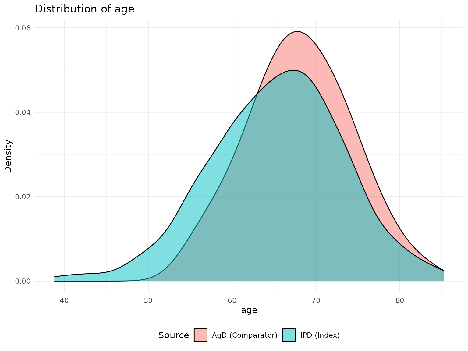

print(p2)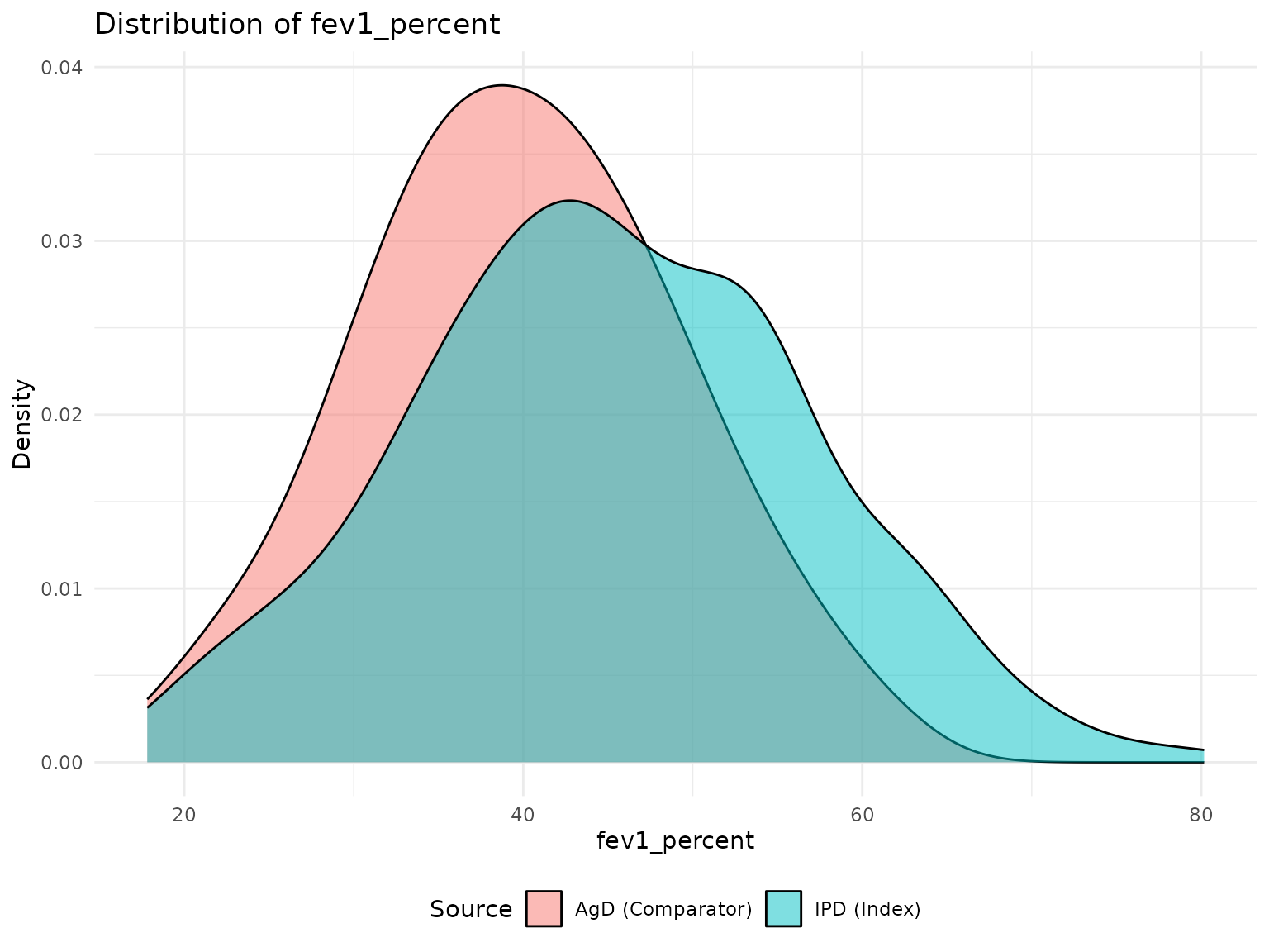

print(p3)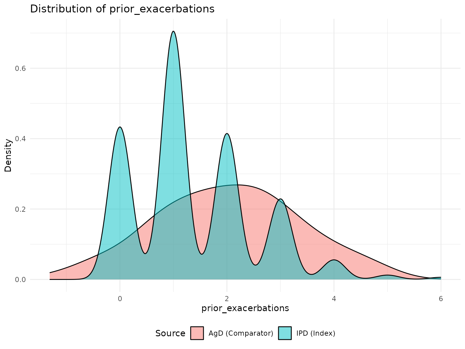

Step 4: Fit ML-UMR Models

Model with SPFA

fit_spfa <- mlumr(
  data = network,
  spfa = TRUE,
  prior_intercept = prior_normal(0, 2),  # Log-rate scale
  prior_beta = prior_normal(0, 1),
  iter_warmup = 1000,
  iter_sampling = 2000,
  chains = 4,
  seed = 123
)

print(fit_spfa)
summary(fit_spfa)

Model with Relaxed SPFA

fit_relaxed <- mlumr(
  data = network,
  spfa = FALSE,
  prior_intercept = prior_normal(0, 2),
  prior_beta = prior_normal(0, 1),
  iter_warmup = 1000,
  iter_sampling = 2000,
  chains = 4,
  seed = 123
)

Step 5: Extract Rate Ratios

Marginal Rate Ratios

For Poisson outcomes, marginal_effects() returns rate ratios:

# Extract rate ratios in both populations
effects <- marginal_effects(fit_spfa, population = "both", effect_type = "rate_ratio")
print(effects)

Interpretation:

Rate Ratio < 1: Treatment A has lower exacerbation rate (beneficial)
Rate Ratio = 1: No difference between treatments
Rate Ratio > 1: Treatment A has higher rate (harmful)

Absolute Rate Predictions

# Predicted exacerbation rates for each treatment in each population
preds <- predict(fit_spfa, population = "both", treatment = "both")
print(preds)

# These are rates (events per unit time)
# Multiply by follow-up duration for expected event counts

Forest Plot

plot_marginal_effects_forest(fit_spfa, effect_type = "rate_ratio") +
  geom_vline(xintercept = 1, linetype = "dashed") +
  labs(x = "Rate Ratio (Treatment A / Treatment B)")

Step 6: Model Comparison

# Compare SPFA vs Relaxed models
comparison <- compare_models(fit_spfa, fit_relaxed)

# If prior exacerbations are a stronger predictor for one treatment,
# the relaxed model may fit better

Clinical Interpretation

Understanding Rate Ratios

# Example output (hypothetical values):
#
# Effect        Population   Mean    SD    2.5%   97.5%
# RATE_RATIO    Index        0.72   0.08   0.57   0.89
# RATE_RATIO    Comparator   0.68   0.10   0.50   0.88
#
# Interpretation:
# - Rate Ratio of 0.72 means Treatment A reduces exacerbation rate by 28%
# - (1 - 0.72) * 100 = 28% reduction vs Treatment B
# - Consistent across populations (similar RR in both)
# - 95% CrI excludes 1, suggesting statistical significance

Clinical Significance

For COPD exacerbations: - Rate ratio < 0.85: Considered clinically meaningful - Rate ratio 0.70-0.80: Moderate reduction (typical for effective therapies) - Rate ratio < 0.70: Strong reduction

Number Needed to Treat (NNT)

# Calculate NNT from rate difference
# If baseline rate = 1.5 events/year
# And rate ratio = 0.72
# Treatment A rate = 1.5 * 0.72 = 1.08
# Rate difference = 1.5 - 1.08 = 0.42 events/year prevented

# NNT = 1 / rate_difference = 1 / 0.42 = 2.4
# Meaning: Treat ~2.4 patients for 1 year to prevent 1 exacerbation

Special Considerations for Rate Data

1. Exposure Time Handling

The Poisson model accounts for varying follow-up:

# IPD: Each patient has individual follow-up time
# AgD: Total exposure = sum of all patient follow-up times

# The model estimates rates (events/time), not counts
# This allows valid comparisons despite different follow-up durations

2. Overdispersion

The Poisson model assumes variance equals mean. In practice, rates may be overdispersed (variance > mean). Consider:

# Check for overdispersion in IPD
observed_var <- var(ipd_data$exacerbation_count)
expected_var <- mean(ipd_data$exacerbation_count)
dispersion_ratio <- observed_var / expected_var

cat("Dispersion ratio:", round(dispersion_ratio, 2), "\n")
cat("If >> 1, consider negative binomial model (not yet implemented)\n")

3. Zero-Inflation

If many patients have zero events, consider whether: - Sample size is adequate - Follow-up is long enough - The Poisson model is appropriate

# Proportion of zeros
prop_zero <- mean(ipd_data$exacerbation_count == 0)
cat("Proportion with zero events:", round(prop_zero * 100, 1), "%\n")

# High zero proportion (>50%) may indicate need for zero-inflated model

4. Prior Selection for Log-Rate

# Priors are on the log-rate scale
# If baseline rate ~1 event/year, log(1) = 0
# N(0, 2) prior on intercept covers rates from ~0.02 to ~50

# For coefficients:
# N(0, 1) allows rate ratios from ~0.05 to ~20 per unit change
# More restrictive: N(0, 0.5) for rate ratios ~0.2 to ~5

5. Reporting Results

Standard reporting for rate outcomes:

# Report:
# 1. Absolute rates in each population
#    "The adjusted exacerbation rate was 0.85/year (95% CrI: 0.70-1.02)
#     for Treatment A and 1.18/year (95% CrI: 0.98-1.40) for Treatment B"
#
# 2. Rate ratio with confidence interval
#    "The rate ratio was 0.72 (95% CrI: 0.57-0.89)"
#
# 3. Rate difference (optional)
#    "Treatment A prevented 0.33 exacerbations per patient-year
#     (95% CrI: 0.15-0.52)"

Example: Multiple Sclerosis Relapse Rates

Here’s a template for MS relapse data:

# IPD structure for MS relapse study
ms_ipd <- data.frame(
  patient_id = 1:200,
  treatment = "Treatment_A",
  relapse_count = rpois(200, lambda = 0.3),  # Annual relapse count
  followup_years = runif(200, 0.5, 2),       # 6 months to 2 years
  age = rnorm(200, 40, 10),
  edss_baseline = rnorm(200, 3, 1.5),        # Disability score
  prior_relapses = rpois(200, lambda = 1)    # Prior year relapses
)

# AgD structure
ms_agd <- data.frame(
  treatment = "Treatment_B",
  total_relapses = 45,           # Sum of relapses
  total_exposure = 180,          # Person-years
  age_mean = 42, age_sd = 9,
  edss_baseline_mean = 3.5, edss_baseline_sd = 1.3,
  prior_relapses_mean = 1.2, prior_relapses_sd = 0.8
)

Summary

This vignette demonstrated:

Setting up ML-UMR for count/rate outcomes with Poisson likelihood
Handling exposure time for varying follow-up durations
Using outcome_r (total events) and outcome_E (total exposure) for AgD
Interpreting rate ratios and converting to clinical metrics
Mixing continuous and binary covariates in the integration

For binary outcomes, see the main tutorial vignette. For continuous outcomes, see the “Continuous Outcomes” vignette.

Session Information

sessionInfo()
#> R version 4.5.2 (2025-10-31)
#> Platform: x86_64-pc-linux-gnu
#> Running under: Ubuntu 24.04.3 LTS
#> 
#> Matrix products: default
#> BLAS:   /usr/lib/x86_64-linux-gnu/openblas-pthread/libblas.so.3 
#> LAPACK: /usr/lib/x86_64-linux-gnu/openblas-pthread/libopenblasp-r0.3.26.so;  LAPACK version 3.12.0
#> 
#> locale:
#>  [1] LC_CTYPE=C.UTF-8       LC_NUMERIC=C           LC_TIME=C.UTF-8       
#>  [4] LC_COLLATE=C.UTF-8     LC_MONETARY=C.UTF-8    LC_MESSAGES=C.UTF-8   
#>  [7] LC_PAPER=C.UTF-8       LC_NAME=C              LC_ADDRESS=C          
#> [10] LC_TELEPHONE=C         LC_MEASUREMENT=C.UTF-8 LC_IDENTIFICATION=C   
#> 
#> time zone: UTC
#> tzcode source: system (glibc)
#> 
#> attached base packages:
#> [1] stats     graphics  grDevices utils     datasets  methods   base     
#> 
#> other attached packages:
#> [1] ggplot2_4.0.2 dplyr_1.2.0   mlumr_0.1.0  
#> 
#> loaded via a namespace (and not attached):
#>  [1] sass_0.4.10         utf8_1.2.6          generics_0.1.4     
#>  [4] lattice_0.22-7      digest_0.6.39       magrittr_2.0.4     
#>  [7] evaluate_1.0.5      grid_4.5.2          RColorBrewer_1.1-3 
#> [10] mvtnorm_1.3-3       fastmap_1.2.0       jsonlite_2.0.0     
#> [13] Matrix_1.7-4        rngWELL_0.10-10     purrr_1.2.1        
#> [16] scales_1.4.0        stabledist_0.7-2    randtoolbox_2.0.5  
#> [19] numDeriv_2016.8-1.1 textshaping_1.0.4   jquerylib_0.1.4    
#> [22] cli_3.6.5           rlang_1.1.7         pspline_1.0-21     
#> [25] gsl_2.1-9           withr_3.0.2         cachem_1.1.0       
#> [28] yaml_2.3.12         tools_4.5.2         copula_1.1-6       
#> [31] vctrs_0.7.1         R6_2.6.1            stats4_4.5.2       
#> [34] lifecycle_1.0.5     ADGofTest_0.3       fs_1.6.6           
#> [37] ragg_1.5.0          pcaPP_2.0-5         pkgconfig_2.0.3    
#> [40] desc_1.4.3          pkgdown_2.2.0       pillar_1.11.1      
#> [43] bslib_0.10.0        gtable_0.3.6        glue_1.8.0         
#> [46] systemfonts_1.3.1   xfun_0.56           tibble_3.3.1       
#> [49] tidyselect_1.2.1    knitr_1.51          farver_2.1.2       
#> [52] htmltools_0.5.9     labeling_0.4.3      rmarkdown_2.30     
#> [55] compiler_4.5.2      S7_0.2.1

mlumr package

2026-02-06