Continuous Outcomes: Mean Difference Analysis
mlumr package
2026-02-06
Source:vignettes/continuous_outcomes.Rmd
continuous_outcomes.RmdOverview
This vignette demonstrates how to use ML-UMR for continuous outcomes where the treatment effect is measured as a mean difference (MD). Common applications include: - Change from baseline in HbA1c (diabetes) - Blood pressure reduction (hypertension) - Pain scores (analgesics) - Quality of life measures - Cognitive function scores
Clinical Scenario
Consider comparing two treatments for type 2 diabetes:
- Treatment A (index): New oral antidiabetic agent - IPD available from a Phase 3 trial
- Treatment B (comparator): Standard of care - Only published aggregate data available
The primary endpoint is change from baseline in HbA1c (%) at 24 weeks.
Step 1: Prepare the Data
Simulate Realistic Clinical Trial Data
set.seed(2024)

# --- Index Treatment (IPD) ---
n_index <- 250

# Patient characteristics
ipd_data <- data.frame(
  patient_id = 1:n_index,
  treatment = "Treatment_A",

  # Baseline characteristics (prognostic factors)
  age = rnorm(n_index, mean = 58, sd = 10),
  baseline_hba1c = rnorm(n_index, mean = 8.5, sd = 1.2),
  diabetes_duration = rgamma(n_index, shape = 4, rate = 0.5),
  bmi = rnorm(n_index, mean = 31, sd = 5)
)

# True model parameters for Treatment A
alpha_A <- -1.2  # Baseline effect
beta_age <- -0.01  # Older patients respond slightly less
beta_hba1c <- -0.15  # Higher baseline = more reduction
beta_duration <- 0.02  # Longer disease = less response
sigma <- 0.8  # Residual SD

# Generate outcomes
ipd_data$hba1c_change <- with(ipd_data, {
  alpha_A +
    beta_age * (age - 58) +
    beta_hba1c * (baseline_hba1c - 8.5) +
    beta_duration * (diabetes_duration - 8) +
    rnorm(n_index, 0, sigma)
})

# --- Comparator Treatment (AgD) ---
# Different population (younger, lower baseline HbA1c)
n_comparator <- 200

# True parameters for Treatment B
alpha_B <- -0.8  # Less effective baseline

# Simulate comparator population (not observed)
age_comp <- rnorm(n_comparator, mean = 52, sd = 9)
hba1c_comp <- rnorm(n_comparator, mean = 7.8, sd = 1.0)
duration_comp <- rgamma(n_comparator, shape = 3, rate = 0.5)

y_comp <- alpha_B +
  beta_age * (age_comp - 58) +
  beta_hba1c * (hba1c_comp - 8.5) +
  beta_duration * (duration_comp - 8) +
  rnorm(n_comparator, 0, sigma)

# Create aggregate summary (what's published)
agd_data <- data.frame(
  study = "Comparator_Study",
  treatment = "Treatment_B",

  # Outcome summary
  mean_change = mean(y_comp),
  se_change = sd(y_comp) / sqrt(n_comparator),

  # Covariate summaries
  age_mean = mean(age_comp),
  age_sd = sd(age_comp),
  baseline_hba1c_mean = mean(hba1c_comp),
  baseline_hba1c_sd = sd(hba1c_comp),
  diabetes_duration_mean = mean(duration_comp),
  diabetes_duration_sd = sd(duration_comp)
)

# Display summary
cat("IPD Summary (Treatment A):\n")
#> IPD Summary (Treatment A):
cat("  N =", n_index, "\n")
#>   N = 250
cat("  Mean HbA1c change =", round(mean(ipd_data$hba1c_change), 2), "%\n")
#>   Mean HbA1c change = -1.22 %
cat("  Age (mean/SD):", round(mean(ipd_data$age), 1), "/",
    round(sd(ipd_data$age), 1), "\n")
#>   Age (mean/SD): 58.4 / 9.9
cat("  Baseline HbA1c (mean/SD):", round(mean(ipd_data$baseline_hba1c), 2), "/",
    round(sd(ipd_data$baseline_hba1c), 2), "\n\n")
#>   Baseline HbA1c (mean/SD): 8.57 / 1.15

cat("AgD Summary (Treatment B):\n")
#> AgD Summary (Treatment B):
cat("  N =", n_comparator, "\n")
#>   N = 200
cat("  Mean HbA1c change =", round(agd_data$mean_change, 2), "%\n")
#>   Mean HbA1c change = -0.67 %
cat("  Age (mean/SD):", round(agd_data$age_mean, 1), "/",
    round(agd_data$age_sd, 1), "\n")
#>   Age (mean/SD): 53.1 / 8.1
cat("  Baseline HbA1c (mean/SD):", round(agd_data$baseline_hba1c_mean, 2), "/",
    round(agd_data$baseline_hba1c_sd, 2), "\n")
#>   Baseline HbA1c (mean/SD): 7.75 / 0.96
Assess Population Imbalance
# The comparator population is younger with lower baseline HbA1c
# This imbalance could bias a naive indirect comparison

cat("\nPopulation Differences:\n")
#>
#> Population Differences:
cat("  Age difference:", round(mean(ipd_data$age) - agd_data$age_mean, 1), "years\n")
#>   Age difference: 5.3 years
cat("  Baseline HbA1c difference:",
    round(mean(ipd_data$baseline_hba1c) - agd_data$baseline_hba1c_mean, 2), "%\n")
#>   Baseline HbA1c difference: 0.82 %
Step 2: Set Up ML-UMR Data Structures
Prepare IPD
ipd <- set_ipd_unanchored(
  data = ipd_data,
  treatment = "treatment",
  outcome = "hba1c_change",
  covariates = c("age", "baseline_hba1c", "diabetes_duration"),
  likelihood = "normal"  # Continuous outcome
)

print(ipd)
#> $data
#> # A tibble: 250 × 6
#>    .study    .trt        .outcome   age baseline_hba1c diabetes_duration
#>    <chr>     <chr>          <dbl> <dbl>          <dbl>             <dbl>
#>  1 IPD_Study Treatment_A   -0.213  67.8          10.6              10.2
#>  2 IPD_Study Treatment_A   -1.65   62.7           8.71              4.53
#>  3 IPD_Study Treatment_A   -1.85   56.9           9.73              5.31
#>  4 IPD_Study Treatment_A   -0.255  55.9           8.17             17.9
#>  5 IPD_Study Treatment_A   -0.645  69.6           8.83             12.0
#>  6 IPD_Study Treatment_A   -1.67   70.9           6.61              9.47
#>  7 IPD_Study Treatment_A   -1.73   63.3           8.68              9.47
#>  8 IPD_Study Treatment_A   -2.27   56.7           8.31              4.67
#>  9 IPD_Study Treatment_A   -1.14   45.8           9.16              3.94
#> 10 IPD_Study Treatment_A   -1.50   46.8           7.12              8.69
#> # ℹ 240 more rows
#>
#> $n
#> [1] 250
#>
#> $n_events
#> [1] NA
#>
#> $treatment
#> [1] "Treatment_A"
#>
#> $covariates
#> [1] "age"               "baseline_hba1c"    "diabetes_duration"
#>
#> $likelihood
#> [1] "normal"
#>
#> $type
#> [1] "ipd"
#>
#> attr(,"class")
#> [1] "ipd_unanchored" "list"
Prepare AgD
agd <- set_agd_unanchored(
  data = agd_data,
  treatment = "treatment",
  outcome_y = "mean_change",      # Mean outcome
  outcome_se = "se_change",       # Standard error
  cov_means = c("age_mean", "baseline_hba1c_mean", "diabetes_duration_mean"),
  cov_sds = c("age_sd", "baseline_hba1c_sd", "diabetes_duration_sd"),
  cov_types = c("continuous", "continuous", "continuous"),
  likelihood = "normal"
)

print(agd)
#> $data
#> # A tibble: 1 × 10
#>   .study    .trt            .y    .se age_mean age_sd baseline_hba1c_mean
#>   <chr>     <chr>        <dbl>  <dbl>    <dbl>  <dbl>               <dbl>
#> 1 AgD_Study Treatment_B -0.665 0.0559     53.1   8.14                7.75
#> # ℹ 3 more variables: baseline_hba1c_sd <dbl>, diabetes_duration_mean <dbl>,
#> #   diabetes_duration_sd <dbl>
#>
#> $n
#> [1] NA
#>
#> $n_events
#> [1] NA
#>
#> $treatment
#> [1] "Treatment_B"
#>
#> $covariates
#> [1] "age"               "baseline_hba1c"    "diabetes_duration"
#>
#> $cov_info
#> $cov_info$age
#> $cov_info$age$mean_col
#> [1] "age_mean"
#>
#> $cov_info$age$sd_col
#> [1] "age_sd"
#>
#> $cov_info$age$type
#> [1] "continuous"
#>
#>
#> $cov_info$baseline_hba1c
#> $cov_info$baseline_hba1c$mean_col
#> [1] "baseline_hba1c_mean"
#>
#> $cov_info$baseline_hba1c$sd_col
#> [1] "baseline_hba1c_sd"
#>
#> $cov_info$baseline_hba1c$type
#> [1] "continuous"
#>
#>
#> $cov_info$diabetes_duration
#> $cov_info$diabetes_duration$mean_col
#> [1] "diabetes_duration_mean"
#>
#> $cov_info$diabetes_duration$sd_col
#> [1] "diabetes_duration_sd"
#>
#> $cov_info$diabetes_duration$type
#> [1] "continuous"
#>
#>
#>
#> $likelihood
#> [1] "normal"
#>
#> $type
#> [1] "agd"
#>
#> attr(,"class")
#> [1] "agd_unanchored" "list"
Combine Data
network <- combine_unanchored(ipd, agd)
print(network)
#> Unanchored Comparison Data
#> ===========================
#>
#> Likelihood: normal
#>
#> Index treatment (IPD): Treatment_A
#>   - N = 250
#>   - Continuous outcome
#>
#> Comparator treatment (AgD): Treatment_B
#>   - Continuous outcome (AgD summary)
#>
#> Covariates ( 3 ): age, baseline_hba1c, diabetes_duration
#>
#> Integration points: Not yet added (use add_integration_unanchored())
Step 3: Add Integration Points
For continuous covariates, we use normal distributions parameterized by the reported means and SDs:
network <- add_integration_unanchored(
  network,
  n_int = 100,  # More points for 3 covariates
  age = distr(qnorm, mean = age_mean, sd = age_sd),
  baseline_hba1c = distr(qnorm, mean = baseline_hba1c_mean, sd = baseline_hba1c_sd),
  diabetes_duration = distr(qnorm, mean = diabetes_duration_mean, sd = diabetes_duration_sd)
)
#> Computing correlation matrix from IPD...
#> Added 100 integration points for AgD

print(network)
#> Unanchored Comparison Data
#> ===========================
#>
#> Likelihood: normal
#>
#> Index treatment (IPD): Treatment_A
#>   - N = 250
#>   - Continuous outcome
#>
#> Comparator treatment (AgD): Treatment_B
#>   - Continuous outcome (AgD summary)
#>
#> Covariates ( 3 ): age, baseline_hba1c, diabetes_duration
#>
#> Integration points: 100 (QMC with Gaussian copula)
Visualize Population Differences
p1 <- plot_covariate_distribution(network, "age") +
  labs(title = "Age Distribution")
p2 <- plot_covariate_distribution(network, "baseline_hba1c") +
  labs(title = "Baseline HbA1c Distribution")

print(p1)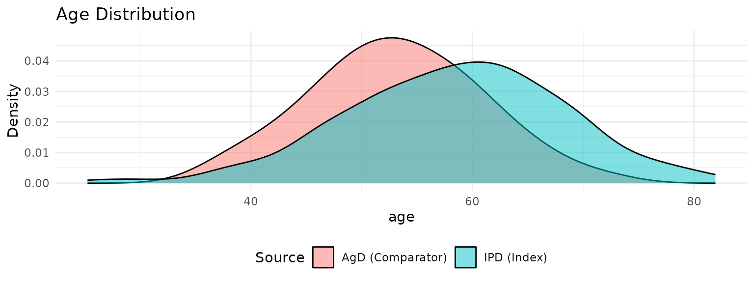
print(p2)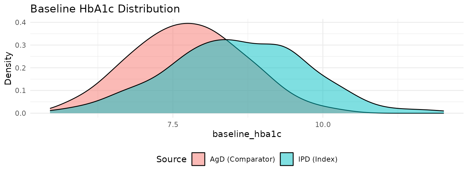
Step 4: Fit ML-UMR Models
Model with SPFA
The SPFA model assumes prognostic factors have the same effect on outcomes regardless of treatment:
fit_spfa <- mlumr(
  data = network,
  spfa = TRUE,
  prior_intercept = prior_normal(0, 5),  # Weakly informative
  prior_beta = prior_normal(0, 2),        # Moderate shrinkage
  iter_warmup = 1000,
  iter_sampling = 2000,
  chains = 4,
  seed = 123
)

print(fit_spfa)
Model with Relaxed SPFA
The relaxed model allows treatment-specific covariate effects (effect modification):
fit_relaxed <- mlumr(
  data = network,
  spfa = FALSE,
  prior_intercept = prior_normal(0, 5),
  prior_beta = prior_normal(0, 2),
  iter_warmup = 1000,
  iter_sampling = 2000,
  chains = 4,
  seed = 123
)

print(fit_relaxed)
Step 5: Extract and Interpret Results
Mean Difference Estimates
# Extract mean differences in both populations
effects <- marginal_effects(fit_spfa, population = "both", effect_type = "md")
print(effects)
Interpretation:
- MD in Index Population: Treatment A vs B effect if both treatments were given to the IPD population (older, higher baseline HbA1c)
- MD in Comparator Population: Treatment A vs B effect if both treatments were given to the AgD population (younger, lower baseline HbA1c)
Forest Plot
plot_marginal_effects_forest(fit_spfa, effect_type = "md") +
  labs(x = "Mean Difference in HbA1c Change (%)")
Step 6: Model Comparison
# Compare SPFA vs Relaxed models
comparison <- compare_models(fit_spfa, fit_relaxed)
Decision criteria:
- If SPFA model has lower DIC: Use SPFA model (simpler, more precise)
- If Relaxed model has lower DIC by >5: Evidence of effect modification; consider using relaxed model or investigating further
Clinical Interpretation
Understanding the Results
Population-Adjusted Effects: Unlike naive comparisons, ML-UMR adjusts for differences in age, baseline HbA1c, and disease duration between populations.
-
Two Target Populations:
- Index population effect: What would happen if comparator patients received Treatment A instead?
- Comparator population effect: What would happen if index patients received Treatment B instead?
Clinical Significance: A mean difference of 0.3-0.5% in HbA1c is typically considered clinically meaningful.
Example Results Interpretation
# Example output (hypothetical values):
#
# Effect    Population   Mean    SD    2.5%   97.5%
# MD        Index       -0.42   0.15  -0.71  -0.13
# MD        Comparator  -0.38   0.18  -0.73  -0.04
#
# Interpretation:
# - Treatment A reduces HbA1c by approximately 0.4% more than Treatment B
# - Effect is consistent across populations (similar MD in both)
# - 95% CrI excludes 0, suggesting statistical significance
# - Effect size is clinically meaningful (>0.3%)
Special Considerations for Continuous Outcomes
1. Residual Variance
The normal likelihood model estimates a residual standard deviation
(sigma) from the IPD. This captures within-treatment
variability not explained by covariates.
2. Prior Selection
For continuous outcomes, priors should be calibrated to the outcome scale:
# If HbA1c change typically ranges from -3 to +1:
# - Intercept: N(0, 2) covers plausible range
# - Beta: N(0, 1) allows moderate covariate effects

# More informative if you have prior knowledge:
prior_intercept = prior_normal(-1, 1)  # Expect negative change
prior_beta = prior_normal(0, 0.5) # Small covariate effects4. Missing Data
Handle missing covariates before analysis:
# Check for missingness
sum(!complete.cases(ipd_data[, c("age", "baseline_hba1c")]))

# Options:
# 1. Complete case analysis (default in set_ipd_unanchored)
# 2. Multiple imputation (pre-process data before mlumr)
Summary
This vignette demonstrated:
- Setting up ML-UMR for continuous outcomes with normal likelihood
- Using
outcome_y(mean) andoutcome_se(standard error) for AgD - Interpreting mean difference estimates in different populations
- Accounting for population differences in prognostic factors
For binary outcomes, see the main tutorial vignette. For count/rate outcomes, see the “Count and Rate Outcomes” vignette.
Session Information
sessionInfo()
#> R version 4.5.2 (2025-10-31)
#> Platform: x86_64-pc-linux-gnu
#> Running under: Ubuntu 24.04.3 LTS
#>
#> Matrix products: default
#> BLAS:   /usr/lib/x86_64-linux-gnu/openblas-pthread/libblas.so.3
#> LAPACK: /usr/lib/x86_64-linux-gnu/openblas-pthread/libopenblasp-r0.3.26.so;  LAPACK version 3.12.0
#>
#> locale:
#>  [1] LC_CTYPE=C.UTF-8       LC_NUMERIC=C           LC_TIME=C.UTF-8
#>  [4] LC_COLLATE=C.UTF-8     LC_MONETARY=C.UTF-8    LC_MESSAGES=C.UTF-8
#>  [7] LC_PAPER=C.UTF-8       LC_NAME=C              LC_ADDRESS=C
#> [10] LC_TELEPHONE=C         LC_MEASUREMENT=C.UTF-8 LC_IDENTIFICATION=C
#>
#> time zone: UTC
#> tzcode source: system (glibc)
#>
#> attached base packages:
#> [1] stats     graphics  grDevices utils     datasets  methods   base
#>
#> other attached packages:
#> [1] ggplot2_4.0.2 dplyr_1.2.0   mlumr_0.1.0
#>
#> loaded via a namespace (and not attached):
#>  [1] sass_0.4.10         utf8_1.2.6          generics_0.1.4
#>  [4] lattice_0.22-7      digest_0.6.39       magrittr_2.0.4
#>  [7] evaluate_1.0.5      grid_4.5.2          RColorBrewer_1.1-3
#> [10] mvtnorm_1.3-3       fastmap_1.2.0       jsonlite_2.0.0
#> [13] Matrix_1.7-4        rngWELL_0.10-10     purrr_1.2.1
#> [16] scales_1.4.0        stabledist_0.7-2    randtoolbox_2.0.5
#> [19] numDeriv_2016.8-1.1 textshaping_1.0.4   jquerylib_0.1.4
#> [22] cli_3.6.5           rlang_1.1.7         pspline_1.0-21
#> [25] gsl_2.1-9           withr_3.0.2         cachem_1.1.0
#> [28] yaml_2.3.12         tools_4.5.2         copula_1.1-6
#> [31] vctrs_0.7.1         R6_2.6.1            stats4_4.5.2
#> [34] lifecycle_1.0.5     ADGofTest_0.3       fs_1.6.6
#> [37] ragg_1.5.0          pcaPP_2.0-5         pkgconfig_2.0.3
#> [40] desc_1.4.3          pkgdown_2.2.0       pillar_1.11.1
#> [43] bslib_0.10.0        gtable_0.3.6        glue_1.8.0
#> [46] systemfonts_1.3.1   xfun_0.56           tibble_3.3.1
#> [49] tidyselect_1.2.1    knitr_1.51          farver_2.1.2
#> [52] htmltools_0.5.9     labeling_0.4.3      rmarkdown_2.30
#> [55] compiler_4.5.2      S7_0.2.1