Survival outcomes: a disconnected network under proportional hazards • cpaic

library(cpaic)
library(ggplot2)
library(survival)
#> Warning: package 'survival' was built under R version 4.6.1
set.seed(2026)

This vignette is the time-to-event counterpart of vignette("continuous-outcomes"): the same problem (a treatment network that is disconnected and whose trials enrolled different populations), the same two routes (frequentist two-stage, one-stage Bayesian), but on a non-collapsible scale and with an exact survival likelihood. Read the continuous vignette first if you want the easy version; almost everything that is simple there is subtle here.

The data here are entirely simulated. The clinical setting (heart failure with reduced ejection fraction) is used only for its vocabulary, because guideline-directed heart failure therapy is genuinely additive: drugs are stacked onto a background regimen. No data, effect estimate, or result below is taken from any publication, and the interaction pattern we impose is invented for the illustration. We set the true parameter values ourselves, which is what lets us check whether each method recovers them.

The clinical question

The outcome is time to cardiovascular death or heart failure hospitalization, so the summary measure is a hazard ratio (HR) on a proportional-hazards model.

Write Std for standard background care (the inactive comparator) and use four add-on components: B (a beta-blocker), M (a mineralocorticoid receptor antagonist), S (an SGLT2 inhibitor), and A (an angiotensin receptor-neprilysin inhibitor). The trials fall into two groups that share no treatment:

Sub-network 1, legacy trials adding one drug to standard care: Std vs Std+B, Std vs Std+M.
Sub-network 2, contemporary trials adding one more drug on top of a beta-blocker and an MRA: B+M vs B+M+S, B+M vs B+M+A.

No trial links the two. The decision maker still has to ask: what does a patient on a beta-blocker gain by adding an MRA and an SGLT2 inhibitor? That is B+M+S versus Std+B, and it crosses the gap. No trial measured it.

The effect modifier is renal function, egfr_c = (eGFR $-$ 60) / 10, in units of 10 mL/min/1.73m $^2$ above 60. The contemporary trials enrolled patients with worse renal function than the legacy ones, and (in our simulated truth) the MRA’s benefit shrinks as eGFR rises while the SGLT2 inhibitor’s does not. That imbalance is exactly what population adjustment is for.

The model

The component-additive ML-NMR gives every individual the hazard

$h_i(t) \;=\; h_0(t)\, \exp(\eta_i), \qquad \eta_i \;=\; \mu_{s(i)} \;+\; x_i^\top b \;+\; C_{t(i)}^\top \bigl(\beta + \Gamma x_i\bigr),$

so the conditional log hazard ratio of treatment $t$ versus $u$ in a population with effect-modifier value $x$ is $\theta_t(x) - \theta_u(x)$ with $\theta_t(x) = C_t^\top(\beta + \Gamma x)$ . As in the continuous case the estimand is population-specific, and relative_effects() will insist on newdata.

The baseline hazard, and why the likelihood is exact

cpaic writes the baseline hazard as a positive combination of basis functions, $h_0(t) = \sum_k \lambda_k \, B_k(t)$ , and evaluates both the basis and its exact integral $\int_0^t B_k(u)\,du$ . Two choices:

`baseline`	$h_0(t)$	Controlled by
`"piecewise"` (default)	a step function, one free level per interval	`cut_points` (`NULL` gives the exponential model)
`"mspline"`	a continuous cubic M-spline; the cumulative hazard uses the exact integrated I-spline basis, with a simplex constraint on the coefficients (Phillippo, Sadek, et al. 2025)	`n_basis`

Because the integrated basis is available in closed form, the cumulative hazard $H_i(t) = \exp(\eta_i)\int_0^t h_0(u)\,du$ is exact, and so is every likelihood contribution. There is no numerical quadrature over time anywhere in the model. The construction follows the general-likelihood ML-NMR of Phillippo, Dias, et al. (2025), specialized to a component-additive treatment effect.

Write $H(t) = \exp(\eta)\int_0^t h_0(u)\,du$ for the cumulative hazard and let $a$ be the patient’s entry time (.entry, zero unless they entered late). Everything is conditioned on survival to $a$ , so every contribution is written through the entry-conditioned cumulative hazard

$\Lambda(t) \;=\; H(t) - H(a), \qquad\text{so that}\qquad \frac{S(t)}{S(a)} \;=\; e^{-\Lambda(t)} .$

The four status codes then contribute

$\ell = \begin{cases} -\Lambda(t) & \text{status } 0, \text{ right-censored} \\ \log h(t) - \Lambda(t) & \text{status } 1, \text{ observed event} \\ \log\bigl(1 - e^{-\Lambda(t)}\bigr) & \text{status } 2, \text{ left-censored} \\ \log\bigl(e^{-\Lambda(\text{start})} - e^{-\Lambda(t)}\bigr) & \text{status } 3, \text{ interval-censored} \end{cases}$

The placement of the conditioning matters and is easy to get wrong. For an observed event or a right-censored observation you may add $+H(a)$ afterwards and get the same answer, because the contribution is linear in the cumulative hazard. For a left-censored observation you may not: $\bigl(1 - S(t)\bigr) / S(a)$ is not a probability and can exceed one, whereas $1 - S(t)/S(a)$ is the correct term. The conditioning has to go inside. .entry is optional (a missing column means everyone enters at zero), and interval-censored rows take their lower endpoint from .start.

Aggregate survival data must be pseudo-IPD

This is the part people get wrong, so it gets its own subsection.

An aggregate survival arm must be supplied to cmlnmr() as reconstructed pseudo-individual rows: one row per (pseudo-)patient with a .time and a .y status, exactly the object multinma::set_agd_surv() expects, and exactly what the Guyot algorithm produces from a digitized Kaplan-Meier curve (Guyot et al. 2012). Event counts plus person-time will not do, and cpaic rejects them.

The reason is not fussiness. A published arm is a mixture over its covariate distribution, and the model has to integrate the individual likelihood over that mixture. The tempting shortcut, “expected events = total person-time times the mean hazard”, is exact within a homogeneous group and wrong for a mixture, because hazard and person-time are negatively correlated: high-hazard patients leave the risk set early, so most of the person-time is contributed by low-hazard patients, and multiplying it by the average hazard over-counts events. Formally $\mathbb{E}[hT] = \mathbb{E}[h]\mathbb{E}[T] + \mathrm{Cov}(h, T)$ with $\mathrm{Cov}(h,T) < 0$ .

Two equal groups with hazards 0.1 and 0.4, followed to time 10:

h   <- c(0.1, 0.4)          # constant hazards in the two halves
w   <- c(0.5, 0.5)          # equal mixing weights
tau <- 10                   # administrative censoring

exact       <- sum(w * (1 - exp(-h * tau)))          # events per person
person_time <- sum(w * (1 - exp(-h * tau)) / h)      # E[min(T, tau)]
approx      <- person_time * sum(w * h)              # person-time x mean hazard

round(c(exact = exact, approximation = approx,
        inflation = approx / exact), 4)
#>         exact approximation     inflation 
#>        0.8069        1.0969        1.3594

The person-time approximation is biased upward by 36%, on a completely ordinary amount of hazard heterogeneity. That is why the aggregate survival API takes pseudo-IPD and integrates the likelihood row by row.

Simulating the evidence

treatments <- c("Std", "Std+B", "Std+M", "B+M", "B+M+S", "B+M+A")
Cmat <- build_C_matrix(treatments, inactive = "Std")
Cmat
#>       A B M S
#> Std   0 0 0 0
#> Std+B 0 1 0 0
#> Std+M 0 0 1 0
#> B+M   0 1 1 0
#> B+M+S 0 1 1 1
#> B+M+A 1 1 1 0

# TRUTH (conditional log hazard ratios at eGFR 60).
beta_true  <- c(A = -0.20, B = -0.35, M = -0.30, S = -0.26)
# Invented interactions: the MRA loses ground as renal function improves;
# the SGLT2 inhibitor gains a little; the beta-blocker is unmodified.
gamma_true <- c(A =  0.05, B =  0.00, M =  0.18, S = -0.08)
stopifnot(identical(names(beta_true), colnames(Cmat)))

The interesting consequence, which we will have to recover: the MRA’s component effect is $-0.30 + 0.18x$ , so at eGFR 50 ( $x = -1$ ) it is a log hazard ratio of $-0.48$ , and at eGFR 70 ( $x = +1$ ) it is only $-0.12$ . Adding the SGLT2 inhibitor contributes a further $-0.26 - 0.08x$ , which barely moves. In a preserved-renal-function population the MRA has almost nothing left to give and the SGLT2 inhibitor supplies the benefit; in a chronic-kidney-disease population the MRA is carrying most of it. One hazard ratio cannot say both.

The data-generating model is a Weibull proportional-hazards model with an increasing baseline hazard. Delayed entry is simulated properly, by drawing the event time from the distribution conditional on survival past the entry time; this is what left truncation is, and it is why a naive analysis that ignores .entry is biased.

lambda <- 0.022; kshape <- 1.2; prognostic <- -0.35; maxt <- 36

gen_arm <- function(study, trt, n, mu0, egfr_mean, egfr_sd = 18,
                    p_late = 0, dropout = 0.008) {
  x   <- (rnorm(n, egfr_mean, egfr_sd) - 60) / 10
  tc  <- Cmat[trt, ]
  eta <- mu0 + prognostic * x +
    sum(tc * beta_true) + sum(tc * gamma_true) * x
  entry <- rep(0, n)
  if (p_late > 0) entry <- ifelse(runif(n) < p_late, runif(n, 1, 8), 0)
  u  <- runif(n)
  # Weibull PH, drawn conditional on T > entry: that is what left truncation is.
  tt <- (entry^kshape - log(u) / (lambda * exp(eta)))^(1 / kshape)
  cn <- pmin(entry + rexp(n, dropout), maxt)     # dropout + administrative
  data.frame(.study = study, .trt = trt,
             .time = pmin(tt, cn), .y = as.integer(tt <= cn),
             .entry = entry, egfr_c = x)
}

ipd <- rbind(
  gen_arm("HF-2", "Std",   150,  0.00, 66),   # sub-network 1
  gen_arm("HF-2", "Std+M", 150,  0.00, 66),
  gen_arm("HF-3", "B+M",   150,  0.00, 58),   # sub-network 2
  gen_arm("HF-3", "B+M+S", 150,  0.00, 58),
  gen_arm("HF-4", "B+M",   150,  0.00, 54),
  gen_arm("HF-4", "B+M+S", 150,  0.00, 54))
ipd$.entry <- NULL                             # nobody enters late: column optional

published <- rbind(
  gen_arm("HF-1", "Std",   50,  0.10, 68),
  gen_arm("HF-1", "Std+B", 50,  0.10, 68),
  gen_arm("HF-5", "B+M",   50, -0.05, 62),
  gen_arm("HF-5", "B+M+A", 50, -0.05, 62),
  gen_arm("HF-6", "Std",   50,  0.05, 72, p_late = 0.30),  # 30% enter late
  gen_arm("HF-6", "Std+M", 50,  0.05, 72, p_late = 0.30))

Now we throw away what a publication does not give us. From published we keep the Kaplan-Meier curve (here, the pseudo-IPD rows that a Guyot reconstruction would return) and the baseline table (an arm-level mean and SD of eGFR). The individual covariate values are discarded.

covs <- do.call(rbind, lapply(
  split(published, list(published$.study, published$.trt), drop = TRUE),
  function(d) data.frame(.study = d$.study[1], .trt = d$.trt[1],
                         egfr_c_mean = mean(d$egfr_c),
                         egfr_c_sd   = sd(d$egfr_c))))

agd <- merge(published[, c(".study", ".trt", ".time", ".y", ".entry")],
             covs, by = c(".study", ".trt"), sort = FALSE)
str(agd)
#> 'data.frame':    300 obs. of  7 variables:
#>  $ .study     : chr  "HF-1" "HF-1" "HF-1" "HF-1" ...
#>  $ .trt       : chr  "Std" "Std" "Std" "Std" ...
#>  $ .time      : num  0.659 1.303 27.633 12.206 19.33 ...
#>  $ .y         : int  1 1 1 1 1 0 1 1 0 1 ...
#>  $ .entry     : num  0 0 0 0 0 0 0 0 0 0 ...
#>  $ egfr_c_mean: num  0.573 0.573 0.573 0.573 0.573 ...
#>  $ egfr_c_sd  : num  1.83 1.83 1.83 1.83 1.83 ...

Every aggregate row carries its arm’s covariate summary, repeated. That is all the model needs: it integrates each row’s likelihood over the covariate distribution implied by the mean and SD.

c(IPD_rows = nrow(ipd), AgD_pseudo_IPD_rows = nrow(agd),
  IPD_events = sum(ipd$.y), AgD_events = sum(agd$.y),
  delayed_entry_rows = sum(agd$.entry > 0))
#>            IPD_rows AgD_pseudo_IPD_rows          IPD_events          AgD_events 
#>                 900                 300                 485                 156 
#>  delayed_entry_rows 
#>                  30

Covariate balance

mean_by_study <- function(d, col) {
  m <- tapply(d[[col]], d$.study, mean)
  data.frame(study = names(m), eGFR = 60 + 10 * as.numeric(m))
}
balance <- rbind(
  cbind(mean_by_study(ipd, "egfr_c"), source = "IPD"),
  cbind(mean_by_study(agd, "egfr_c_mean"), source = "AgD"))
balance$subnetwork <- ifelse(balance$study %in% c("HF-1", "HF-2", "HF-6"), 1, 2)
knitr::kable(balance[order(balance$subnetwork, balance$study), ], digits = 1,
             row.names = FALSE,
             caption = "Mean eGFR by trial: the imbalance across the gap")

Mean eGFR by trial: the imbalance across the gap
study	eGFR	source	subnetwork
HF-1	66.4	AgD	1
HF-2	66.5	IPD	1
HF-6	72.3	AgD	1
HF-3	59.4	IPD	2
HF-4	52.3	IPD	2
HF-5	64.2	AgD	2

The legacy trials run around 66 to 72 mL/min and the contemporary ones around 54 to 62, a gap of roughly 10 mL/min. Since the MRA’s log hazard ratio moves by $+0.18$ per 10 mL/min, that gap on its own is worth about 0.18 on the log scale, against an MRA effect of $-0.30$ . The imbalance is more than half the size of the effect we are trying to measure.

The observed evidence

keep <- c(".study", ".trt", ".time", ".y", ".entry")
all_dat <- rbind(cbind(ipd[, setdiff(keep, ".entry")], .entry = 0),
                 agd[, keep])

km_curve <- function(d) {
  s <- survfit(Surv(.entry, .time, .y) ~ 1, data = d)
  data.frame(.study = d$.study[1], .trt = d$.trt[1],
             time = c(0, s$time), surv = c(1, s$surv))
}
km <- do.call(rbind, lapply(
  split(all_dat, list(all_dat$.study, all_dat$.trt), drop = TRUE), km_curve))
km$subnetwork <- ifelse(km$.study %in% c("HF-1", "HF-2", "HF-6"),
                        "1: legacy (Std backbone)",
                        "2: contemporary (B+M backbone)")

ggplot(km, aes(time, surv, color = .trt)) +
  geom_step(linewidth = 0.8) +
  facet_wrap(~ subnetwork + .study, nrow = 2) +
  scale_y_continuous(limits = c(0, 1)) +
  labs(x = "Months", y = "Event-free survival", color = NULL,
       title = "Observed Kaplan-Meier curves",
       subtitle = paste("HF-2, HF-3, HF-4 are IPD; HF-1, HF-5, HF-6 are",
                        "reconstructed from published KM curves.",
                        "No treatment label appears in both rows.")) +
  theme_minimal(base_size = 10) +
  theme(legend.position = "bottom")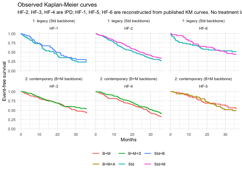

plot of chunk km

Look across the two rows: no treatment label is shared. That is the disconnection, and no amount of Kaplan-Meier plotting will fix it.

Setting up the data

As in the continuous vignette, the frequentist route wants contrast-level aggregate data. For a survival outcome the “published” contrast is the trial’s own log hazard ratio, which we obtain from each aggregate trial’s reconstructed data (and, for HF-6, with its delayed entry handled).

study_loghr <- function(s, t1, t2) {
  d <- all_dat[all_dat$.study == s, ]
  d$arm <- as.integer(d$.trt == t1)
  f <- coxph(Surv(.entry, .time, .y) ~ arm, data = d)
  data.frame(studlab = s, treat1 = t1, treat2 = t2,
             TE = unname(coef(f)), seTE = unname(sqrt(diag(vcov(f)))))
}
contrasts <- rbind(
  study_loghr("HF-1", "Std+B", "Std"),
  study_loghr("HF-2", "Std+M", "Std"),
  study_loghr("HF-3", "B+M+S", "B+M"),
  study_loghr("HF-4", "B+M+S", "B+M"),
  study_loghr("HF-5", "B+M+A", "B+M"),
  study_loghr("HF-6", "Std+M", "Std"))
knitr::kable(contrasts, digits = 3, row.names = FALSE,
             caption = "Unadjusted within-trial log hazard ratios, as published")

Unadjusted within-trial log hazard ratios, as published
studlab	treat1	treat2	TE	seTE
HF-1	Std+B	Std	-0.178	0.249
HF-2	Std+M	Std	-0.208	0.148
HF-3	B+M+S	B+M	-0.256	0.173
HF-4	B+M+S	B+M	-0.234	0.155
HF-5	B+M+A	B+M	0.104	0.302
HF-6	Std+M	Std	0.160	0.294

HF-2 and HF-6 both compare Std+M with Std, and they do not agree. They also enrolled populations 6 mL/min apart in mean eGFR, which under our simulated truth is worth about 0.11 on the log hazard scale. The two-stage bridge will call that disagreement heterogeneity; the one-stage model will call it effect modification and use it. (With only 50 pseudo-patients per arm, HF-6 is also just noisy, and it would be dishonest to pretend the raw numbers separate those two explanations. Nothing below leans on them.)


net <- cpaic_network(contrasts, ipd = ipd, sm = "HR", family = "survival",
                     ipd_time = ".time", ipd_status = ".y",
                     ipd_covariates = "egfr_c", inactive = "Std")
net
#> cpaic component network
#>   Summary measure:   HR
#>   Treatments:        6
#>   Components:        4 (A, B, M, S)
#>   AgD comparisons:   6
#>   Reference:         Std
#>   Inactive:          Std
#>   IPD studies:       3 (survival; 900 patients)
#>   Connected:         FALSE | components bridgeable: TRUE
cpaic_connectivity(net)
#> cpaic connectivity
#>   Connected network: FALSE
#>   Sub-networks:      2
#>     [1] 3 treatments
#>     [2] 3 treatments
#>   Bridging components: B, M
#>   Component design:  rank(X) = 4 / 4 components -> all component effects identified
#>   Estimable effects: 5 / 5 vs Std

The network plot puts both halves of the problem in one picture.

plot(net)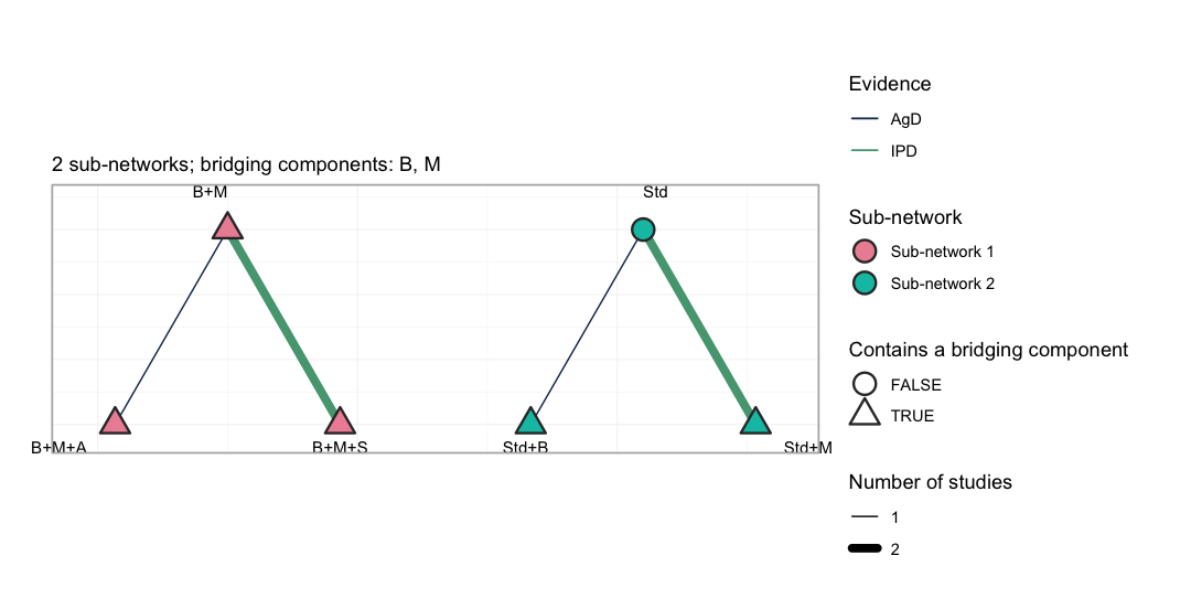

plot of chunk netplot

Each sub-network is drawn on its own circle, so the disconnection is not something the reader has to take on trust: no edge crosses from the left group to the right. Edge color separates the trials that carry individual patient data from those that do not, and the outlined nodes are the treatments containing a bridging component. The subtitle names those components, and cpaic_connectivity() above names them too: B and M, the beta-blocker and the MRA, are the only treatment components that occur on both sides of the gap. They are the entire basis on which the additive component model reconnects the network.

The target population

target_ckd  <- c(egfr_c = -1)   # eGFR 50: chronic kidney disease
target_pres <- c(egfr_c =  1)   # eGFR 70: preserved renal function

# The chronic-kidney-disease target again, as the one-row data frame that the
# Bayesian model's `newdata` argument takes.
target <- data.frame(egfr_c = -1)

theta <- function(trt, x) sum(Cmat[trt, ] * (beta_true + gamma_true * x))
truth <- function(t1, t2, x) theta(t1, x) - theta(t2, x)
data.frame(
  target = c("eGFR 50", "eGFR 70"),
  `B+M vs Std+B (true HR)`   = exp(c(truth("B+M", "Std+B", -1),
                                     truth("B+M", "Std+B",  1))),
  `B+M+S vs Std+B (true HR)` = exp(c(truth("B+M+S", "Std+B", -1),
                                     truth("B+M+S", "Std+B",  1))),
  check.names = FALSE)
#>    target B+M vs Std+B (true HR) B+M+S vs Std+B (true HR)
#> 1 eGFR 50              0.6187834                0.5168513
#> 2 eGFR 70              0.8869204                0.6312836

Fitting

Route 1: the frequentist two-stage bridge

cstc() fits a Cox model per IPD study with treatment, prognostic main effects, and treatment-by-effect-modifier interactions, the modifiers centered at the target. Its treatment coefficient is the conditional log hazard ratio at the target covariate values. cmaic() reweights each IPD study to the target and fits an unadjusted weighted Cox model, so its coefficient is the marginal log hazard ratio in the target population (Signorovitch et al. 2010; Phillippo et al. 2018).

stc_ckd  <- cstc(net,  target = target_ckd, effect_modifiers = "egfr_c")
maic_ckd <- cmaic(net, target = target_ckd, effect_modifiers = "egfr_c",
                  n_boot = 200, seed = 7)
relative_effects(stc_ckd,  reference = "Std+B")
#> Relative effects (HR, back-transformed)
#>  treatment comparator estimate    se lower upper      z     p
#>        B+M      Std+B    0.818 0.169 0.587 1.140 -1.187 0.235
#>      B+M+A      Std+B    0.908 0.361 0.448 1.841 -0.268 0.789
#>      B+M+S      Std+B    0.621 0.219 0.404 0.953 -2.180 0.029
#>        Std      Std+B    1.195 0.269 0.705 2.023  0.662 0.508
#>      Std+M      Std+B    0.977 0.318 0.524 1.821 -0.072 0.943
relative_effects(maic_ckd, reference = "Std+B")
#> Relative effects (HR, back-transformed)
#>  treatment comparator estimate    se lower upper      z     p
#>        B+M      Std+B    0.874 0.138 0.667 1.145 -0.981 0.327
#>      B+M+A      Std+B    0.969 0.332 0.506 1.858 -0.093 0.926
#>      B+M+S      Std+B    0.703 0.183 0.490 1.007 -1.924 0.054
#>        Std      Std+B    1.195 0.249 0.733 1.946  0.714 0.475
#>      Std+M      Std+B    1.044 0.285 0.597 1.823  0.150 0.881
effective_sample_size(maic_ckd)
#>     HF-2     HF-3     HF-4 
#> 156.3300 231.1447 294.8349

forest(stc_ckd, reference = "Std+B")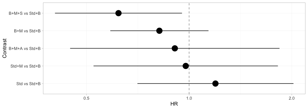

plot of chunk freq-forest

The bridged network, adjusted to the chronic-kidney-disease target, on one axis. Every contrast comes back with an estimate, because the two-stage bridge asks only whether the component design has full rank, and it has. Hold that thought: the Bayesian model below will refuse three of these five, and it will be right to.

Which trials actually pay for a given answer is a separate question, and plot_edge_influence() answers it.

plot_edge_influence(stc_ckd, treatment = "B+M+S")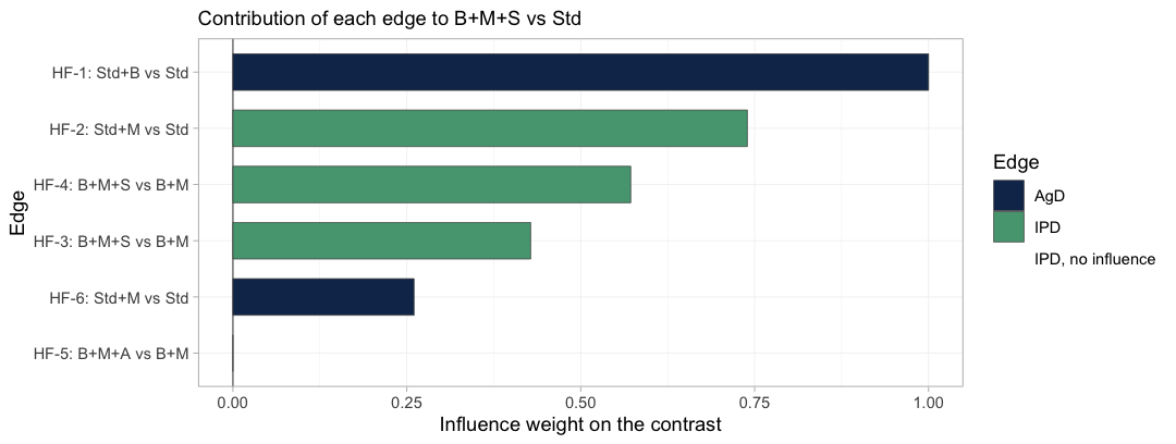

plot of chunk edge-influence

Each bar is the weight with which one observed edge enters the estimate of B+M+S versus Std. That contrast decomposes into the components B, M and S, so it draws on trials from both sub-networks: HF-1 is the only source of B and carries the whole weight of it, while HF-3 and HF-4 supply S, and HF-2 and HF-6 supply M. This is the bridge doing its work, and no Kaplan-Meier plot shows it. HF-5 carries exactly zero weight, because the ARNI component A does not enter this contrast at all.

The diagnostic bites hardest on IPD edges. An IPD trial with zero influence on the contrast you care about cannot move that contrast however carefully you reweight it, and no MAIC weight diagnostic will tell you so: the effective sample size can look perfectly healthy while the edge is contributing nothing. Such edges are drawn in red and named in the caption; there are none here.

Route 2: the one-stage Bayesian model

We fit a piecewise-exponential baseline and a cubic M-spline baseline, then compare them. Note what agd is: pseudo-IPD rows plus arm-level covariate summaries. Nothing else.

fit_pw <- cmlnmr(ipd, agd, effect_modifiers = "egfr_c", inactive = "Std",
                 family = "survival", baseline = "piecewise",
                 cut_points = c(9, 18, 27), n_int = 8,
                 chains = 4, iter_warmup = 400, iter_sampling = 400,
                 seed = 2026)
fit_pw
#> cpaic: component-additive ML-NMR (Bayesian, survival)
#>   Treatment effects: fixed
#>   Effect modifiers: egfr_c [normal]
#>   Component effects below are at the covariate origin (x = 0).
#>   For a target population use relative_effects(fit, newdata = ...).
#> 
#>  component estimate    se  lower  upper
#>          A   -0.170 0.394 -1.053  0.538
#>          B   -0.299 0.262 -0.816  0.206
#>          M   -0.218 0.131 -0.478  0.032
#>          S   -0.347 0.129 -0.596 -0.092

fit_ms <- cmlnmr(ipd, agd, effect_modifiers = "egfr_c", inactive = "Std",
                 family = "survival", baseline = "mspline", n_basis = 5,
                 n_int = 8,
                 chains = 4, iter_warmup = 400, iter_sampling = 400,
                 seed = 2026)
#> Chain 4 Informational Message: The current Metropolis proposal is about to be rejected because of the following issue:
#> Chain 4 Exception: cpaic_survival_mspline_b5f2792f65_model_namespace::log_prob: coefficients[1] is not a valid simplex. sum(coefficients[1]) = nan, but should be 1 (in '/var/folders/2h/yqztgsf96gsbkqn60cymgsjr0000gn/T/RtmpIoTyq5/model-20663f38bdd4.stan', line 143, column 2 to column 48)
#> Chain 4 If this warning occurs sporadically, such as for highly constrained variable types like covariance matrices, then the sampler is fine,
#> Chain 4 but if this warning occurs often then your model may be either severely ill-conditioned or misspecified.
#> Chain 4
#> Chain 4 Informational Message: The current Metropolis proposal is about to be rejected because of the following issue:
#> Chain 4 Exception: cpaic_survival_mspline_b5f2792f65_model_namespace::log_prob: coefficients[1] is not a valid simplex. sum(coefficients[1]) = nan, but should be 1 (in '/var/folders/2h/yqztgsf96gsbkqn60cymgsjr0000gn/T/RtmpIoTyq5/model-20663f38bdd4.stan', line 143, column 2 to column 48)
#> Chain 4 If this warning occurs sporadically, such as for highly constrained variable types like covariance matrices, then the sampler is fine,
#> Chain 4 but if this warning occurs often then your model may be either severely ill-conditioned or misspecified.
#> Chain 4
#> Chain 4 Informational Message: The current Metropolis proposal is about to be rejected because of the following issue:
#> Chain 4 Exception: cpaic_survival_mspline_b5f2792f65_model_namespace::log_prob: coefficients[1] is not a valid simplex. sum(coefficients[1]) = nan, but should be 1 (in '/var/folders/2h/yqztgsf96gsbkqn60cymgsjr0000gn/T/RtmpIoTyq5/model-20663f38bdd4.stan', line 143, column 2 to column 48)
#> Chain 4 If this warning occurs sporadically, such as for highly constrained variable types like covariance matrices, then the sampler is fine,
#> Chain 4 but if this warning occurs often then your model may be either severely ill-conditioned or misspecified.
#> Chain 4
#> Chain 4 Informational Message: The current Metropolis proposal is about to be rejected because of the following issue:
#> Chain 4 Exception: cpaic_survival_mspline_b5f2792f65_model_namespace::log_prob: coefficients[1] is not a valid simplex. sum(coefficients[1]) = nan, but should be 1 (in '/var/folders/2h/yqztgsf96gsbkqn60cymgsjr0000gn/T/RtmpIoTyq5/model-20663f38bdd4.stan', line 143, column 2 to column 48)
#> Chain 4 If this warning occurs sporadically, such as for highly constrained variable types like covariance matrices, then the sampler is fine,
#> Chain 4 but if this warning occurs often then your model may be either severely ill-conditioned or misspecified.
#> Chain 4
#> Chain 4 Informational Message: The current Metropolis proposal is about to be rejected because of the following issue:
#> Chain 4 Exception: cpaic_survival_mspline_b5f2792f65_model_namespace::log_prob: coefficients[1] is not a valid simplex. sum(coefficients[1]) = nan, but should be 1 (in '/var/folders/2h/yqztgsf96gsbkqn60cymgsjr0000gn/T/RtmpIoTyq5/model-20663f38bdd4.stan', line 143, column 2 to column 48)
#> Chain 4 If this warning occurs sporadically, such as for highly constrained variable types like covariance matrices, then the sampler is fine,
#> Chain 4 but if this warning occurs often then your model may be either severely ill-conditioned or misspecified.
#> Chain 4
#> Chain 4 Informational Message: The current Metropolis proposal is about to be rejected because of the following issue:
#> Chain 4 Exception: cpaic_survival_mspline_b5f2792f65_model_namespace::log_prob: coefficients[1] is not a valid simplex. sum(coefficients[1]) = nan, but should be 1 (in '/var/folders/2h/yqztgsf96gsbkqn60cymgsjr0000gn/T/RtmpIoTyq5/model-20663f38bdd4.stan', line 143, column 2 to column 48)
#> Chain 4 If this warning occurs sporadically, such as for highly constrained variable types like covariance matrices, then the sampler is fine,
#> Chain 4 but if this warning occurs often then your model may be either severely ill-conditioned or misspecified.
#> Chain 4
#> Chain 4 Informational Message: The current Metropolis proposal is about to be rejected because of the following issue:
#> Chain 4 Exception: cpaic_survival_mspline_b5f2792f65_model_namespace::log_prob: coefficients[1] is not a valid simplex. sum(coefficients[1]) = nan, but should be 1 (in '/var/folders/2h/yqztgsf96gsbkqn60cymgsjr0000gn/T/RtmpIoTyq5/model-20663f38bdd4.stan', line 143, column 2 to column 48)
#> Chain 4 If this warning occurs sporadically, such as for highly constrained variable types like covariance matrices, then the sampler is fine,
#> Chain 4 but if this warning occurs often then your model may be either severely ill-conditioned or misspecified.
#> Chain 4
#> Chain 4 Informational Message: The current Metropolis proposal is about to be rejected because of the following issue:
#> Chain 4 Exception: cpaic_survival_mspline_b5f2792f65_model_namespace::log_prob: coefficients[1] is not a valid simplex. sum(coefficients[1]) = nan, but should be 1 (in '/var/folders/2h/yqztgsf96gsbkqn60cymgsjr0000gn/T/RtmpIoTyq5/model-20663f38bdd4.stan', line 143, column 2 to column 48)
#> Chain 4 If this warning occurs sporadically, such as for highly constrained variable types like covariance matrices, then the sampler is fine,
#> Chain 4 but if this warning occurs often then your model may be either severely ill-conditioned or misspecified.
#> Chain 4
#> Chain 4 Informational Message: The current Metropolis proposal is about to be rejected because of the following issue:
#> Chain 4 Exception: cpaic_survival_mspline_b5f2792f65_model_namespace::log_prob: coefficients[1] is not a valid simplex. sum(coefficients[1]) = nan, but should be 1 (in '/var/folders/2h/yqztgsf96gsbkqn60cymgsjr0000gn/T/RtmpIoTyq5/model-20663f38bdd4.stan', line 143, column 2 to column 48)
#> Chain 4 If this warning occurs sporadically, such as for highly constrained variable types like covariance matrices, then the sampler is fine,
#> Chain 4 but if this warning occurs often then your model may be either severely ill-conditioned or misspecified.
#> Chain 4
#> Chain 4 Informational Message: The current Metropolis proposal is about to be rejected because of the following issue:
#> Chain 4 Exception: cpaic_survival_mspline_b5f2792f65_model_namespace::log_prob: coefficients[1] is not a valid simplex. sum(coefficients[1]) = nan, but should be 1 (in '/var/folders/2h/yqztgsf96gsbkqn60cymgsjr0000gn/T/RtmpIoTyq5/model-20663f38bdd4.stan', line 143, column 2 to column 48)
#> Chain 4 If this warning occurs sporadically, such as for highly constrained variable types like covariance matrices, then the sampler is fine,
#> Chain 4 but if this warning occurs often then your model may be either severely ill-conditioned or misspecified.
#> Chain 4

Each aggregate row’s likelihood is averaged over n_int quasi-Monte-Carlo points drawn from its arm’s covariate distribution, so the aggregate cost scales with n_int times the number of pseudo-patients. With a single effect modifier a Sobol’ sequence in one dimension is essentially a stratified grid and n_int = 8 integrates a smooth function accurately. Do not copy that number into an analysis with several correlated covariates; the default of 64 exists for a reason, and integration error is cheap to check by refitting with more points. Refitting is in fact the only check here: plot_integration_error(), which traces the error against the number of points for the other outcome families, is not available for a survival model, because an aggregate arm contributes a log_sum_exp of the likelihood over the integration points rather than an integrated mean outcome, and there is no single integrated quantity whose error could be plotted.

fit_re <- cmlnmr(ipd, agd, effect_modifiers = "egfr_c", inactive = "Std",
                 family = "survival", baseline = "mspline", n_basis = 5,
                 n_int = 8, trt_effects = "random",
                 chains = 4, iter_warmup = 400, iter_sampling = 400,
                 seed = 2026, adapt_delta = 0.95)
#> Chain 4 Informational Message: The current Metropolis proposal is about to be rejected because of the following issue:
#> Chain 4 Exception: cpaic_survival_mspline_b5f2792f65_model_namespace::log_prob: coefficients[1] is not a valid simplex. sum(coefficients[1]) = nan, but should be 1 (in '/var/folders/2h/yqztgsf96gsbkqn60cymgsjr0000gn/T/RtmpIoTyq5/model-20663f38bdd4.stan', line 143, column 2 to column 48)
#> Chain 4 If this warning occurs sporadically, such as for highly constrained variable types like covariance matrices, then the sampler is fine,
#> Chain 4 but if this warning occurs often then your model may be either severely ill-conditioned or misspecified.
#> Chain 4
#> Chain 4 Informational Message: The current Metropolis proposal is about to be rejected because of the following issue:
#> Chain 4 Exception: cpaic_survival_mspline_b5f2792f65_model_namespace::log_prob: coefficients[1] is not a valid simplex. sum(coefficients[1]) = nan, but should be 1 (in '/var/folders/2h/yqztgsf96gsbkqn60cymgsjr0000gn/T/RtmpIoTyq5/model-20663f38bdd4.stan', line 143, column 2 to column 48)
#> Chain 4 If this warning occurs sporadically, such as for highly constrained variable types like covariance matrices, then the sampler is fine,
#> Chain 4 but if this warning occurs often then your model may be either severely ill-conditioned or misspecified.
#> Chain 4
#> Chain 4 Informational Message: The current Metropolis proposal is about to be rejected because of the following issue:
#> Chain 4 Exception: cpaic_survival_mspline_b5f2792f65_model_namespace::log_prob: coefficients[1] is not a valid simplex. sum(coefficients[1]) = nan, but should be 1 (in '/var/folders/2h/yqztgsf96gsbkqn60cymgsjr0000gn/T/RtmpIoTyq5/model-20663f38bdd4.stan', line 143, column 2 to column 48)
#> Chain 4 If this warning occurs sporadically, such as for highly constrained variable types like covariance matrices, then the sampler is fine,
#> Chain 4 but if this warning occurs often then your model may be either severely ill-conditioned or misspecified.
#> Chain 4
#> Chain 4 Informational Message: The current Metropolis proposal is about to be rejected because of the following issue:
#> Chain 4 Exception: cpaic_survival_mspline_b5f2792f65_model_namespace::log_prob: coefficients[1] is not a valid simplex. sum(coefficients[1]) = nan, but should be 1 (in '/var/folders/2h/yqztgsf96gsbkqn60cymgsjr0000gn/T/RtmpIoTyq5/model-20663f38bdd4.stan', line 143, column 2 to column 48)
#> Chain 4 If this warning occurs sporadically, such as for highly constrained variable types like covariance matrices, then the sampler is fine,
#> Chain 4 but if this warning occurs often then your model may be either severely ill-conditioned or misspecified.
#> Chain 4
#> Chain 4 Informational Message: The current Metropolis proposal is about to be rejected because of the following issue:
#> Chain 4 Exception: cpaic_survival_mspline_b5f2792f65_model_namespace::log_prob: coefficients[1] is not a valid simplex. sum(coefficients[1]) = nan, but should be 1 (in '/var/folders/2h/yqztgsf96gsbkqn60cymgsjr0000gn/T/RtmpIoTyq5/model-20663f38bdd4.stan', line 143, column 2 to column 48)
#> Chain 4 If this warning occurs sporadically, such as for highly constrained variable types like covariance matrices, then the sampler is fine,
#> Chain 4 but if this warning occurs often then your model may be either severely ill-conditioned or misspecified.
#> Chain 4
#> Chain 4 Informational Message: The current Metropolis proposal is about to be rejected because of the following issue:
#> Chain 4 Exception: cpaic_survival_mspline_b5f2792f65_model_namespace::log_prob: coefficients[1] is not a valid simplex. sum(coefficients[1]) = nan, but should be 1 (in '/var/folders/2h/yqztgsf96gsbkqn60cymgsjr0000gn/T/RtmpIoTyq5/model-20663f38bdd4.stan', line 143, column 2 to column 48)
#> Chain 4 If this warning occurs sporadically, such as for highly constrained variable types like covariance matrices, then the sampler is fine,
#> Chain 4 but if this warning occurs often then your model may be either severely ill-conditioned or misspecified.
#> Chain 4
#> Chain 4 Informational Message: The current Metropolis proposal is about to be rejected because of the following issue:
#> Chain 4 Exception: cpaic_survival_mspline_b5f2792f65_model_namespace::log_prob: coefficients[1] is not a valid simplex. sum(coefficients[1]) = nan, but should be 1 (in '/var/folders/2h/yqztgsf96gsbkqn60cymgsjr0000gn/T/RtmpIoTyq5/model-20663f38bdd4.stan', line 143, column 2 to column 48)
#> Chain 4 If this warning occurs sporadically, such as for highly constrained variable types like covariance matrices, then the sampler is fine,
#> Chain 4 but if this warning occurs often then your model may be either severely ill-conditioned or misspecified.
#> Chain 4
#> Chain 4 Informational Message: The current Metropolis proposal is about to be rejected because of the following issue:
#> Chain 4 Exception: cpaic_survival_mspline_b5f2792f65_model_namespace::log_prob: coefficients[1] is not a valid simplex. sum(coefficients[1]) = nan, but should be 1 (in '/var/folders/2h/yqztgsf96gsbkqn60cymgsjr0000gn/T/RtmpIoTyq5/model-20663f38bdd4.stan', line 143, column 2 to column 48)
#> Chain 4 If this warning occurs sporadically, such as for highly constrained variable types like covariance matrices, then the sampler is fine,
#> Chain 4 but if this warning occurs often then your model may be either severely ill-conditioned or misspecified.
#> Chain 4
#> Chain 4 Informational Message: The current Metropolis proposal is about to be rejected because of the following issue:
#> Chain 4 Exception: cpaic_survival_mspline_b5f2792f65_model_namespace::log_prob: coefficients[1] is not a valid simplex. sum(coefficients[1]) = nan, but should be 1 (in '/var/folders/2h/yqztgsf96gsbkqn60cymgsjr0000gn/T/RtmpIoTyq5/model-20663f38bdd4.stan', line 143, column 2 to column 48)
#> Chain 4 If this warning occurs sporadically, such as for highly constrained variable types like covariance matrices, then the sampler is fine,
#> Chain 4 but if this warning occurs often then your model may be either severely ill-conditioned or misspecified.
#> Chain 4
#> Warning: 2 of 1600 (0.0%) transitions ended with a divergence.
#> See https://mc-stan.org/misc/warnings for details.
#> Warning: 2 divergent transition(s) in cmlnmr(); results may be unreliable (consider
#> higher adapt_delta or more iterations).
fit_re$fit$summary("tau")
#> # A tibble: 1 × 10
#>   variable  mean median    sd   mad     q5   q95  rhat ess_bulk ess_tail
#>   <chr>    <dbl>  <dbl> <dbl> <dbl>  <dbl> <dbl> <dbl>    <dbl>    <dbl>
#> 1 tau[1]   0.254  0.163 0.273 0.169 0.0118 0.800  1.01     350.     343.

Six studies and four components leave two degrees of freedom for heterogeneity, so tau is weakly identified and leans on its half-normal(0, 1) prior. Read it as a sensitivity setting, not as an estimate. We report the M-spline fixed-effect model as primary.

Priors

str(fit_ms$priors)
#> List of 5
#>  $ intercept :List of 3
#>   ..$ distribution: chr "normal"
#>   ..$ location    : num 0
#>   ..$ scale       : num 2.5
#>  $ beta      :List of 3
#>   ..$ distribution: chr "normal"
#>   ..$ location    : num 0
#>   ..$ scale       : num 2.5
#>  $ regression:List of 3
#>   ..$ distribution: chr "normal"
#>   ..$ location    : num 0
#>   ..$ scale       : num 1
#>  $ gamma     :List of 4
#>   ..$ distribution: chr "normal"
#>   ..$ location    : num 0
#>   ..$ scale       : num 1
#>   ..$ df          : num 4
#>  $ tau       :List of 4
#>   ..$ distribution: chr "half-normal"
#>   ..$ location    : num 0
#>   ..$ scale       : num 1
#>   ..$ df          : num 4

The component by effect-modifier prior (gamma) is the load-bearing one. A component whose interaction is informed only by aggregate arms has nothing but this prior holding it up, which is precisely why estimable_effects_at() exists and why we check prior_sensitivity() below.

plot_prior_posterior() is the same statement as a picture: the posterior is the histogram, the prior is the red line, and where the two coincide the data have said nothing.

plot_prior_posterior(fit_ms)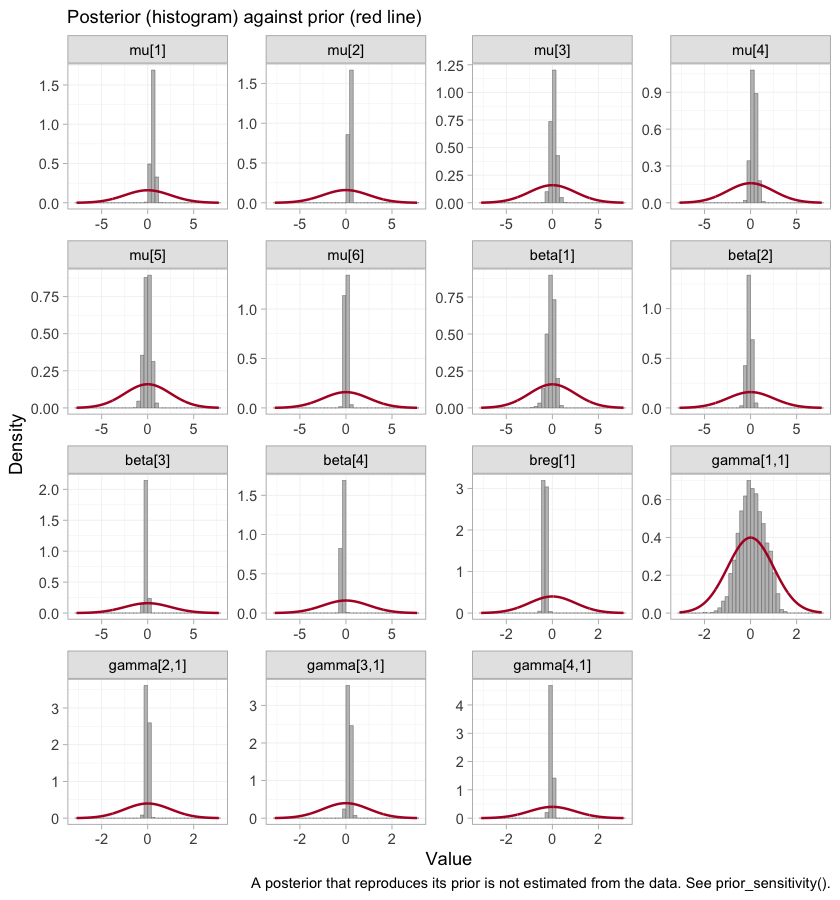

plot of chunk prior-post

plot_prior_posterior(fit_ms, prior = "gamma")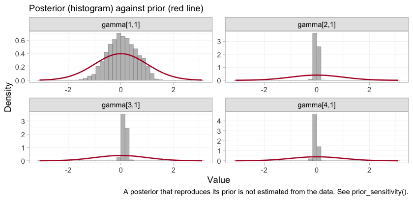

plot of chunk prior-post-gamma

The gamma panels are the four components in the order of colnames(Cmat): A, B, M, S. The ARNI interaction, gamma[1,1], is much the widest of the four, which is what it looks like when no trial varies eGFR against a component within its own arms. The MRA and SGLT2 interactions, gamma[3,1] and gamma[4,1], are identified from within-trial covariate variation and are far tighter than their prior. A narrow posterior is not on its own a license to report a contrast, and the next two sections are about exactly that gap.

Convergence

rbind(
  piecewise = unlist(fit_pw$diagnostics),
  mspline   = unlist(fit_ms$diagnostics),
  random    = unlist(fit_re$diagnostics))
#>           divergences max_treedepth max_rhat
#> piecewise           0             0 1.005617
#> mspline             0             0 1.014945
#> random              2             0 1.010460

The summary is not a substitute for looking at the chains.

plot(fit_ms, type = "trace")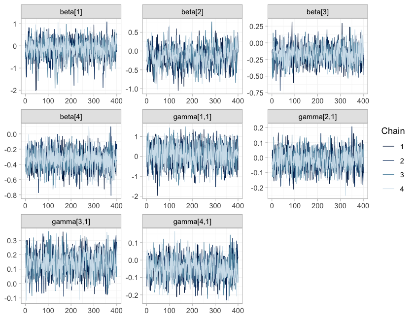

plot of chunk trace

plot(fit_ms, type = "rhat")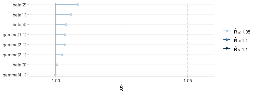

plot of chunk rhat

type = "trace" draws the four chains for the component effects and their interactions; they should overlay each other and show neither drift nor stickiness. type = "rhat" collects the split-Rhat statistics for the same parameters, and the max_rhat column of the table above is the largest of them. These are gatekeepers rather than decoration: had the chains not mixed, nothing below would be worth reading, however narrow the credible intervals looked.

Results

Does the model reproduce the observed curves?

Before reading a hazard ratio off the model, check that the model can reproduce the data it was fitted to. plot_survival() draws the model-implied survival curve for each study arm, averaged over that arm’s own covariate distribution (the individual covariates for an IPD arm, the integration points for an aggregate one), with a credible band that includes the uncertainty in the baseline hazard. geom_km() overlays the observed Kaplan-Meier curve.

plot_survival(fit_ms) + geom_km(fit_ms)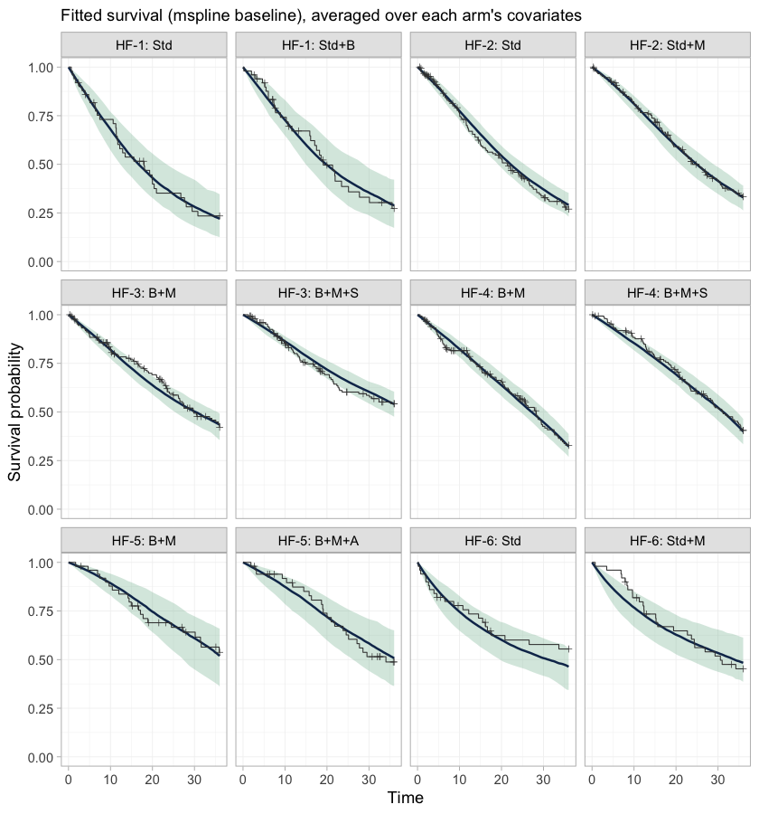

plot of chunk km-overlay

This is the check that the baseline hazards actually fit. Every study carries its own baseline hazard, smoothed by a first-order random-walk prior with a smoothing scale shared across studies, so these twelve panels are not twelve views of one curve: each study’s hazard shape is free to be wrong on its own. A systematic departure of the step function from the band would mean the baseline is too rigid, and would put everything below it in doubt.

One disagreement is guaranteed in advance, and it is HF-6. Thirty percent of its patients enter late; the model conditions on their entry times, and geom_km() draws the ordinary Kaplan-Meier estimator, which does not. The observed curve in those two panels therefore still carries the immortal time that left truncation removes, and sits above the fitted curve early on. That gap is an artifact of the comparison, not a failure of the model.

What is actually estimable?

estimable_effects_at(fit_ms, newdata = data.frame(egfr_c = -1),
                     reference = "Std+B")
#> Estimability of the population-adjusted relative effects
#>   Target population: egfr_c = -1
#>  treatment comparator estimable identified_by              basis
#>        B+M      Std+B      TRUE           IPD first-order screen
#>      B+M+A      Std+B     FALSE          none     not identified
#>      B+M+S      Std+B      TRUE           IPD first-order screen
#>        Std      Std+B     FALSE          none     not identified
#>      Std+M      Std+B     FALSE          none     not identified
#> 
#>   Rows marked "first-order screen" are estimable by the linear criterion, which
#>   is only a design-based screen for them (aggregate identification, or a
#>   survival baseline) and can be optimistic. Check them with prior_sensitivity().
#> 
#>   Rows marked "not identified" carry no first-order information; a number
#>   reported for them would be the prior. relative_effects() returns NA there.

B+M and B+M+S against Std+B are the components M and M + S. Both are identified from IPD (HF-2 for M; HF-3 and HF-4 for S), so their interactions are pinned by within-trial variation in eGFR and the contrasts are estimable in any target population. These two are the cross-gap comparisons we came for.
Std, Std+M and B+M+A are not estimable and come back as NA. Each involves B or A, and each of those components enters through exactly one aggregate two-arm contrast (HF-1 for B, HF-5 for A). A single aggregate contrast pins its effect down at that study’s own covariate mean and nowhere else; it cannot separate the main effect from the interaction. A Bayesian model will still hand you a tidy posterior for B+M+A versus Std+B. That posterior is the prior speaking.

Note that the network is perfectly well reconnected: cpaic_connectivity() above reports rank(X) = 4 out of 4 components, so every component main effect is identified. Reconnection is necessary and not sufficient. Population adjustment needs the interactions too.

relative_effects(fit_ms, reference = "Std+B",
                 newdata = data.frame(egfr_c = -1))
#> Relative effects (HR, back-transformed)
#>   Target population: egfr_c = -1
#>  treatment comparator estimate    se lower upper pr_gt0
#>        B+M      Std+B    0.737 0.169  0.53 1.020  0.031
#>      B+M+A      Std+B       NA    NA    NA    NA     NA
#>      B+M+S      Std+B    0.555 0.209  0.36 0.826  0.003
#>        Std      Std+B       NA    NA    NA    NA     NA
#>      Std+M      Std+B       NA    NA    NA    NA     NA
#>   NA = not uniquely estimable from this component design (see estimable_effects()).

Estimability is a function of the target population, not a property of the network, so it is worth mapping rather than checking at a single point.

plot_estimability(fit_ms, em = "egfr_c", values = seq(-2, 2, by = 0.25),
                  reference = "Std+B")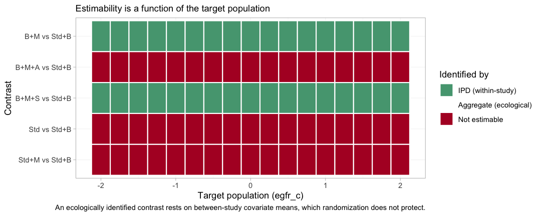

plot of chunk estimability-map

Green is a contrast identified by IPD, from within-trial covariate variation that randomization protects; red is a contrast the design cannot identify at that target at all. The two green bands run the full width of the plot: B+M and B+M+S versus Std+B are estimable in every population on the grid, which is what makes them reportable. The three red bands stay red everywhere. A component carried by a single aggregate contrast is pinned at that trial’s own covariate mean and nowhere else, and no grid point is that mean.

The cross-gap hazard ratio, in two named populations

report <- function(fitobj, t1, x, label) {
  re <- relative_effects(fitobj, reference = "Std+B",
                         newdata = data.frame(egfr_c = x))
  r <- re[re$treatment == t1, ]
  data.frame(target = label, contrast = paste(t1, "vs Std+B"),
             HR = r$estimate, lower = r$lower, upper = r$upper,
             true_HR = exp(truth(t1, "Std+B", x)))
}
res <- rbind(
  report(fit_ms, "B+M",   -1, "eGFR 50"),
  report(fit_ms, "B+M+S", -1, "eGFR 50"),
  report(fit_ms, "B+M",    1, "eGFR 70"),
  report(fit_ms, "B+M+S",  1, "eGFR 70"))
knitr::kable(res, digits = 3, row.names = FALSE,
             caption = "cML-NMR: recovered vs true hazard ratios")

cML-NMR: recovered vs true hazard ratios
target	contrast	HR	lower	upper	true_HR
eGFR 50	B+M vs Std+B	0.737	0.530	1.020	0.619
eGFR 50	B+M+S vs Std+B	0.555	0.360	0.826	0.517
eGFR 70	B+M vs Std+B	0.967	0.734	1.285	0.887
eGFR 70	B+M+S vs Std+B	0.667	0.428	1.015	0.631

All four credible intervals cover the truth, and the pattern the truth encodes is the pattern the model recovers. The MRA’s contribution collapses as renal function improves: B+M versus Std+B goes from a hazard ratio of about 0.74 at eGFR 50 to about 0.97 at eGFR 70. Adding the SGLT2 inhibitor holds the benefit roughly steady across the same range (about 0.56 and 0.67). One population-free hazard ratio would have to average those, and would be wrong for at least one of them.

Now be honest about the precision. Six studies and 641 events do not buy much. Of the four contrasts, only one clearly excludes a hazard ratio of 1: B+M+S versus Std+B in the chronic-kidney-disease population. The B+M interval at eGFR 70 comfortably contains 1, and the other two only just touch it. What this evidence supports is the shape of the effect-modifier relationship, not a decisive claim about either regimen in a preserved-renal-function population. A component by effect-modifier interaction is estimated from covariate variation within a trial, which is expensive information, and this is what the bill looks like. Reporting the point estimates without the intervals would be a lie of omission.

The rest of the network, at the same target

The table above picks out two contrasts. forest() and league_table() report the rest of the network at the same target population, and they keep what they cannot estimate on the page instead of quietly dropping it.

forest(fit_ms, newdata = target, reference = "Std+B")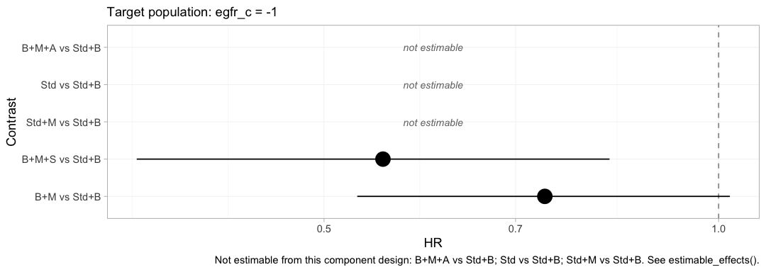

plot of chunk forest-target

Compare this with the frequentist forest above, which drew five estimates from the same network. Three of them are gone, replaced by the words “not estimable”. Nothing has been lost: the three that vanished were never population-adjusted estimates in the first place, only prior-driven ones dressed as estimates, and the plot now says so.

The same effects can be reported one component at a time.

forest(fit_ms, what = "component", newdata = target)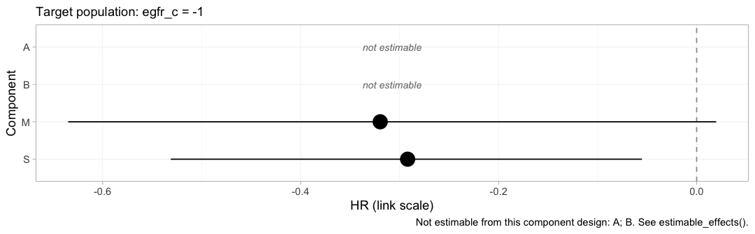

plot of chunk forest-component

Each row is the incremental log hazard ratio of adding one drug to whatever the patient is already taking, evaluated at eGFR 50. This is the level at which the additivity assumption lives, and it is also where the disconnection is repaired: M and S are estimated, A and B are not, and the two treatment contrasts that survive are exactly the two that can be written using only M and S.

knitr::kable(league_table(fit_ms, newdata = target),
             caption = "League table of hazard ratios at eGFR 50 (row vs column)")

League table of hazard ratios at eGFR 50 (row vs column)
	B+M	B+M+A	B+M+S	Std	Std+B	Std+M
B+M	B+M		1.35 (1.06, 1.70)		0.74 (0.53, 1.02)
B+M+A		B+M+A
B+M+S	0.75 (0.59, 0.95)		B+M+S		0.55 (0.36, 0.83)
Std				Std		1.40 (0.98, 1.89)
Std+B	1.40 (0.98, 1.89)		1.88 (1.21, 2.78)		Std+B
Std+M				0.74 (0.53, 1.02)		Std+M

The empty cells are not missing data. They are the pairs this design cannot compare in this population, and a league table that filled them in with prior-driven numbers would be worse than one that leaves them blank.

Sweeping the target population

Two named populations were a convenience. The estimand is defined at every value of the effect modifier, so vary it and plot the whole family at once.

grid <- seq(-2, 2, by = 0.2)
curve <- do.call(rbind, lapply(grid, function(x) {
  re <- relative_effects(fit_ms, reference = "Std+B",
                         newdata = data.frame(egfr_c = x))
  re <- re[re$treatment %in% c("B+M", "B+M+S"), ]
  data.frame(x = x, treatment = re$treatment, HR = re$estimate,
             lower = re$lower, upper = re$upper)
}))
curve$truth <- exp(mapply(truth, curve$treatment, "Std+B", curve$x))

ggplot(curve, aes(60 + 10 * x, HR, color = treatment, fill = treatment)) +
  geom_hline(yintercept = 1, linewidth = 0.3) +
  geom_ribbon(aes(ymin = lower, ymax = upper), alpha = 0.15, color = NA) +
  geom_line(linewidth = 0.9) +
  geom_line(aes(y = truth), linetype = "22", linewidth = 0.7) +
  scale_y_log10(breaks = c(0.3, 0.4, 0.5, 0.6, 0.8, 1.0, 1.2)) +
  labs(x = "eGFR of the target population (mL/min/1.73 m2)",
       y = "Hazard ratio vs Std+B (log scale)", color = NULL, fill = NULL,
       title = "A population-adjusted hazard ratio is a curve, not a number",
       subtitle = "Solid: cML-NMR posterior mean with 95% CrI. Dashed: the truth.") +
  theme_minimal(base_size = 11) +
  theme(legend.position = "bottom")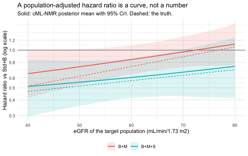

plot of chunk curve

The hierarchy, and what it refuses to rank

A hazard ratio below one is a benefit, so on this scale lower is better, and that has to be said out loud: cpaic_ranks() and rank_probs() both default to the opposite convention.

plot(cpaic_ranks(fit_ms, newdata = target, lower_is_better = TRUE))
#> Warning: Dropped from the hierarchy as not estimable in this target population: B+M,
#> B+M+A, B+M+S, Std+B. Ranking them would rank the prior. See estimable_effects_at().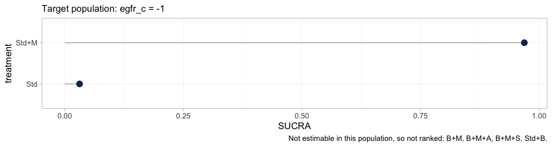

plot of chunk hierarchy

The warning is the figure’s most important output. A treatment hierarchy is anchored at the network reference, here Std, and every treatment containing the beta-blocker is unidentifiable against Std as a population-adjusted effect, for the reason the estimability map gave. Four of the six treatments are therefore dropped, and the hierarchy that survives compares two. It is a thin answer, and it is the honest one.

Pushed one step further, the rankogram declines to draw at all.

tryCatch(
  plot(rank_probs(fit_ms, newdata = target, lower_is_better = TRUE)),
  error = function(e) message("rank_probs() refused: ", conditionMessage(e)))
#> Warning: Dropped from the hierarchy as not estimable in this target population: B+M,
#> B+M+A, B+M+S, Std+B. Ranking them would rank the prior. See estimable_effects_at().
#> rank_probs() refused: Fewer than two elements are estimable in this target population, so no hierarchy can be formed. See estimable_effects_at().

rank_probs() ranks the non-reference treatments, so where cpaic_ranks() had two elements it has one, and it stops. This is not a defect to be worked around with an argument. It is Step 3 of the Wigle et al. hierarchy workflow (Wigle et al. 2026) enforced in code: refine the ranking set to the elements the target population actually identifies, and if too few remain, say so. A rankogram of a prior-driven posterior would look exactly as confident as a real one.

Rank the components instead and the picture comes back, because M and S are both identified from IPD.

plot(rank_probs(fit_ms, newdata = target, what = "component",
                lower_is_better = TRUE))
#> Warning: Dropped from the hierarchy as not estimable in this target population: A, B.
#> Ranking them would rank the prior. See estimable_effects_at().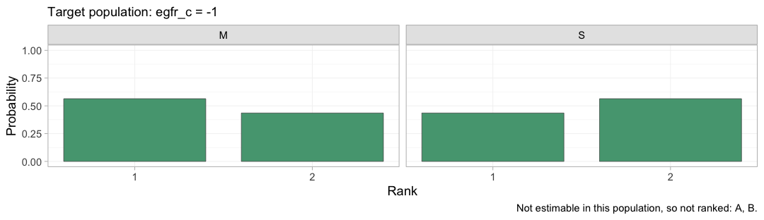

plot of chunk rankogram-component

And because a component’s effect is beta_c + Gamma_c x, its rank is a function of the target population. This is the figure the whole vignette has been building toward.

plot_rank_curve(fit_ms, em = "egfr_c", values = seq(-2, 2, by = 0.25),
                what = "component", lower_is_better = TRUE)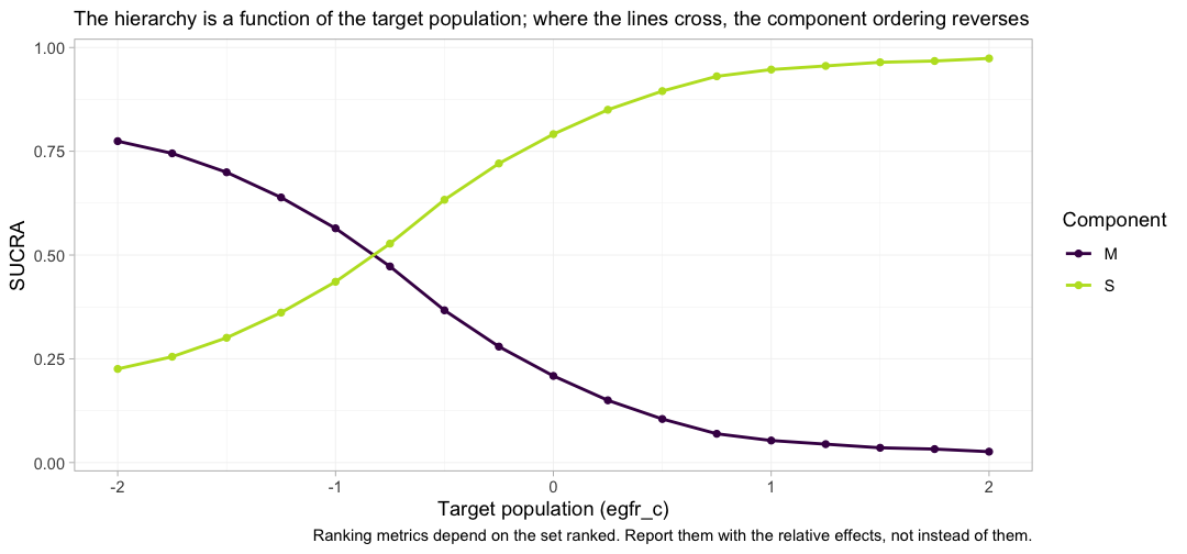

plot of chunk rank-curve

With two components in the ranked set, SUCRA reduces to the posterior probability that a component is the better of the two, and the two curves cross. At the chronic-kidney-disease end of the grid the MRA leads; at the preserved-renal end the SGLT2 inhibitor leads, and by a wide margin. Near eGFR 50 the two are close enough to a coin toss that the ordering carries almost no information, which is what the SUCRA values say and what a bare list of ranks would hide. A component hierarchy quoted without a target population is not a wrong answer to the question; it is not an answer to any question.

Conditional and marginal are not the same thing here

In the continuous vignette cstc() and cmaic() agreed, because the mean difference is collapsible. The hazard ratio is not collapsible (Greenland et al. 1999): averaging individual hazard ratios over a heterogeneous population does not give the population’s hazard ratio, and the marginal hazard ratio is pulled toward the null relative to the conditional one, even when the proportional-hazards model is exactly right and there is no confounding.

So cstc() (conditional) and cmaic() (marginal) estimate different estimands, and both can be correct at once (Remiro-Azócar et al. 2022). cmlnmr() targets the conditional contrast $m^\top(\beta + \Gamma x)$ and therefore lines up with cstc().

We can check this without argument, because we know the truth. Simulate an enormous trial in the target population and read off both quantities:

oracle <- function(t1, t2, x_target, egfr_sd = 18, n = 150000) {
  d <- rbind(gen_arm("O", t1, n, 0, 60 + 10 * x_target, egfr_sd),
             gen_arm("O", t2, n, 0, 60 + 10 * x_target, egfr_sd))
  d$arm <- as.integer(d$.trt == t1)
  d$xc  <- d$egfr_c - x_target     # center the modifier at the target
  c(  # conditional AT x_target: arm coefficient with the interaction in the model
    conditional = coef(coxph(Surv(.time, .y) ~ arm * xc, data = d))[["arm"]],
      # marginal IN the target population: the unadjusted contrast
    marginal    = coef(coxph(Surv(.time, .y) ~ arm, data = d))[["arm"]])
}
set.seed(99)
orc <- oracle("B+M+S", "B+M", -1)     # the SGLT2 edge, in the eGFR-50 population
round(c(orc, simulated_truth = beta_true[["S"]] + gamma_true[["S"]] * -1,
        attenuation_pct = 100 * (1 - abs(orc[["marginal"]]) /
                                   abs(orc[["conditional"]]))), 3)
#>     conditional        marginal simulated_truth attenuation_pct 
#>          -0.181          -0.160          -0.180          11.733

The conditional log hazard ratio recovers the value we simulated. The marginal one is about a tenth smaller in magnitude, and it is smaller by construction, not by mistake: this is a randomized comparison with 150,000 patients per arm and a correctly specified model. The gap is non-collapsibility, and no amount of data will close it.

pick <- function(x, t1) {
  r <- x[x$treatment == t1, ]
  c(HR = r$estimate, lower = r$lower, upper = r$upper)
}
bayes_ckd <- relative_effects(fit_ms, reference = "Std+B",
                              newdata = data.frame(egfr_c = -1))
cm <- rbind(
  data.frame(method = "cSTC (conditional)", estimand = "conditional",
             t(pick(relative_effects(stc_ckd,  reference = "Std+B"), "B+M+S"))),
  data.frame(method = "cMAIC (marginal)", estimand = "marginal",
             t(pick(relative_effects(maic_ckd, reference = "Std+B"), "B+M+S"))),
  data.frame(method = "cML-NMR (conditional)", estimand = "conditional",
             t(pick(bayes_ckd, "B+M+S"))))
cm$true_conditional_HR <- exp(truth("B+M+S", "Std+B", -1))
knitr::kable(cm, digits = 3, row.names = FALSE,
             caption = "B+M+S vs Std+B at eGFR 50: two estimands, three routes")

B+M+S vs Std+B at eGFR 50: two estimands, three routes
method	estimand	HR	lower	upper	true_conditional_HR
cSTC (conditional)	conditional	0.621	0.404	0.953	0.517
cMAIC (marginal)	marginal	0.703	0.490	1.007	0.517
cML-NMR (conditional)	conditional	0.555	0.360	0.826	0.517

There is a second, sharper reason to prefer the conditional route in a component model. The additive structure $\theta_t = C_t^\top\beta$ lives on the linear predictor, and conditional log hazard ratios add up there by construction. Marginal log hazard ratios do not: because the measure is not collapsible, the marginal effect of M + S is not the sum of the marginal effects of M and of S. Feeding cmaic() contrasts into an additive component bridge is therefore an approximation, and one that gets worse the more components you stack. cstc() and cmlnmr() have no such problem. This is a real cost of cmaic() on a non-collapsible scale, and it does not arise for the mean difference.

Prior sensitivity

ps <- prior_sensitivity(fit_ms, newdata = data.frame(egfr_c = -1),
                        prior = "gamma", reference = "Std+B",
                        chains = 2, iter_warmup = 250, iter_sampling = 250)
ps
#> cML-NMR prior sensitivity: gamma prior
#>  treatment comparator estimate tighter looser move_tighter move_looser max_movement
#>        B+M      Std+B   -0.320  -0.314 -0.313        0.006       0.007        0.007
#>      B+M+A      Std+B   -0.527  -0.467 -0.558        0.060       0.031        0.060
#>      B+M+S      Std+B   -0.612  -0.606 -0.608        0.006       0.004        0.006
#>        Std      Std+B    0.134   0.136  0.162        0.002       0.028        0.028
#>      Std+M      Std+B   -0.186  -0.178 -0.150        0.007       0.036        0.036
#>  estimable
#>       TRUE
#>      FALSE
#>       TRUE
#>      FALSE
#>      FALSE

The two estimable contrasts barely move when the interaction prior is halved and doubled. The non-estimable ones are flagged, and their numbers move freely, which is what “prior-driven” looks like from the outside.

Model comparison: which baseline?

loo_pw <- loo::loo(fit_pw)
loo_ms <- loo::loo(fit_ms)
loo::loo_compare(list(piecewise = loo_pw, mspline = loo_ms))
#>      model elpd_diff se_diff p_worse       diag_diff diag_elpd
#>  piecewise       0.0     0.0      NA                          
#>    mspline      -3.3     2.7    0.89 |elpd_diff| < 4
#> 
#> Diagnostic flags present.
#> See ?`loo-glossary` (sections `diag_diff` and `diag_elpd`)
#> or https://mc-stan.org/loo/reference/loo-glossary.html.
dic(fit_pw)
#> Deviance information criterion
#>   DIC: 5915.6
#>   Mean deviance: 5890.5
#>   Effective parameters (pV): 25.2
dic(fit_ms)
#> Deviance information criterion
#>   DIC: 5924.3
#>   Mean deviance: 5894.1
#>   Effective parameters (pV): 30.2
loo::loo_compare(list(mspline_fixed = loo_ms, mspline_random = loo::loo(fit_re)))
#>           model elpd_diff se_diff p_worse       diag_diff diag_elpd
#>   mspline_fixed       0.0     0.0      NA                          
#>  mspline_random      -1.0     0.4    0.99 |elpd_diff| < 4
#> 
#> Diagnostic flags present.
#> See ?`loo-glossary` (sections `diag_diff` and `diag_elpd`)
#> or https://mc-stan.org/loo/reference/loo-glossary.html.

The truth here is Weibull, whose hazard is smooth and monotone. A cubic M-spline can represent that exactly enough; a step function with three interior cut points can only approximate it. Whether leave-one-out cross-validation can see the difference at this sample size is a separate question, and the answer is usually “barely” (Vehtari et al. 2017). Choose the M-spline when you have no positive reason to believe the hazard is piecewise constant, and report the comparison rather than the winner. DIC (Spiegelhalter et al. 2002) is reported alongside because an aggregate arm contributes highly influential observations, which is exactly the situation in which PSIS-LOO’s Pareto $\hat{k}$ diagnostic complains.

A model comparison summarized in one number hides where the two models differ. Passing both dic() objects to plot() gives the dev-dev plot, which compares them one data point at a time.

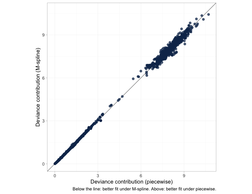
plot(dic(fit_pw), dic(fit_ms), labels = c("piecewise", "M-spline"))

plot of chunk devdev

Each point is one observation’s posterior mean deviance under the two baselines. Points on the line of equality are fitted equally well by both; points below it are fitted better by the M-spline, points above it better by the step function, and the further a point lies from the line the more the choice of baseline matters to it. Read the spread against the numbers above, which are the same verdict arithmetically: the two DIC values differ by a fraction of a point, and the elpd difference is well inside its own standard error. Neither criterion can separate the baselines here, so the choice has to rest on what is plausible about the hazard rather than on what this much data can resolve.

plot_leverage(), the other DIC diagnostic, is not available here and calling it raises an error rather than returning a plot. A leverage plot needs the saturated model, and a censored observation has no saturated reference, so there is no residual deviance to put on the axis; multinma declines the plot for a survival likelihood for the same reason. The dev-dev plot above is the substitute.

What to take away

	Continuous (MD)	Survival (HR)
Collapsible	yes	no
`cstc()` and `cmaic()` target	the same estimand	different estimands
Component effects add up on the	linear predictor, which is also the reporting scale	linear predictor, which is not the marginal scale
Aggregate likelihood	exact at the covariate means	exact, but needs pseudo-IPD and QMC integration
Aggregate input	arm mean and SE	reconstructed KM (time, status) per pseudo-patient

Five things worth keeping.

Aggregate survival arms are pseudo-IPD, full stop. Events and person-time cannot identify an individual likelihood; the shortcut that pretends they can is biased upward by 36% in the two-group example above. Digitize the Kaplan-Meier curve (Guyot et al. 2012) and pass the rows.
The likelihood is exact. Both the hazard basis and its integral are evaluated in closed form, so events, right, left and interval censoring, and delayed entry are all handled without approximation. Nothing is being discretized behind your back.
Estimability is not reconnection. The component design has full rank here, yet Std+M and B+M+A are still not estimable as population-adjusted effects, because B and A each enter through a single aggregate contrast and are pinned only at that study’s covariate mean. NA is the correct output, and estimable_effects_at() is not optional.
Non-collapsibility is not a bug to be tuned away. cstc() and cmlnmr() give you the conditional hazard ratio; cmaic() gives you the marginal one; both are right, and they differ. Decide which one your decision problem wants before you look at the numbers, and remember that only the conditional one is additive across components.
The bridging assumption remains untestable. Reconnecting through M and S requires those component effects, and their interactions with eGFR, to be the same in the legacy and contemporary trials. There is no cross-gap evidence to test that with, and there never will be (Veroniki et al. 2026).

An honest limitation to close on, and it is the biggest one here. The whole analysis assumes proportional hazards conditional on eGFR, and it assumes that hazard ratios (rather than, say, restricted mean survival times) are what the decision needs. Neither is innocuous: the contemporary SGLT2 trials in real heart failure show early separation of the survival curves, which is exactly the pattern a constant conditional hazard ratio cannot represent. A flexible baseline hazard does not rescue this, because the baseline is shared across arms; what would be needed is a time-varying treatment effect, which cpaic does not currently fit. Check proportionality before you trust any of the numbers above, and if it fails, say so rather than reporting a hazard ratio anyway.

References

Greenland, Sander, James M. Robins, and Judea Pearl. 1999. “Confounding and Collapsibility in Causal Inference.” Statistical Science 14 (1): 29–46. https://doi.org/10.1214/ss/1009211805.

Guyot, Patricia, A. E. Ades, Mario J. N. M. Ouwens, and Nicky J. Welton. 2012. “Enhanced Secondary Analysis of Survival Data: Reconstructing the Data from Published Kaplan-Meier Survival Curves.” BMC Medical Research Methodology 12: 9. https://doi.org/10.1186/1471-2288-12-9.

Phillippo, David M., A. E. Ades, Sofia Dias, Stephen Palmer, Keith R. Abrams, and Nicky J. Welton. 2018. “Methods for Population-Adjusted Indirect Comparisons in Health Technology Appraisal.” Medical Decision Making 38 (2): 200–211. https://doi.org/10.1177/0272989X17725740.

Phillippo, David M., Sofia Dias, A. E. Ades, and Nicky J. Welton. 2025. “Multilevel Network Meta-Regression for General Likelihoods: Synthesis of Individual and Aggregate Data with Applications to Survival Analysis.” Journal of the Royal Statistical Society Series A: Statistics in Society, ahead of print. https://doi.org/10.1093/jrsssa/qnaf169.

Phillippo, David M., Ahmed Sadek, Hugo Pedder, and Nicky J. Welton. 2025. Network Meta-Analysis of Survival Outcomes with Non-Proportional Hazards Using Flexible M-splines. https://doi.org/10.48550/arXiv.2509.10383.

Remiro-Azócar, Antonio, Anna Heath, and Gianluca Baio. 2022. “Conflating Marginal and Conditional Treatment Effects: Comments on ‘Assessing the Performance of Population Adjustment Methods for Anchored Indirect Comparisons: A Simulation Study’.” Statistics in Medicine 41 (9): 1541–53. https://doi.org/10.1002/sim.9286.

Signorovitch, James E., Eric Q. Wu, Andrew P. Yu, et al. 2010. “Comparative Effectiveness Without Head-to-Head Trials: A Method for Matching-Adjusted Indirect Comparisons Applied to Psoriasis Treatment with Adalimumab or Etanercept.” PharmacoEconomics 28 (10): 935–45. https://doi.org/10.2165/11538370-000000000-00000.

Spiegelhalter, David J., Nicola G. Best, Bradley P. Carlin, and Angelika van der Linde. 2002. “Bayesian Measures of Model Complexity and Fit.” Journal of the Royal Statistical Society: Series B 64 (4): 583–639. https://doi.org/10.1111/1467-9868.00353.

Vehtari, Aki, Andrew Gelman, and Jonah Gabry. 2017. “Practical Bayesian Model Evaluation Using Leave-One-Out Cross-Validation and WAIC.” Statistics and Computing 27 (5): 1413–32. https://doi.org/10.1007/s11222-016-9696-9.

Veroniki, Areti Angeliki, Georgios Seitidis, Sofia Tsokani, et al. 2026. “Analysing Component Network Meta-Analysis in Disconnected Networks: Guidance for Practice.” BMJ.

Wigle, Augustine, Audrey Béliveau, Adriani Nikolakopoulou, and Lifeng Lin. 2026. Creating Treatment and Component Hierarchies in Component Network Meta-Analysis.