Count outcomes: a disconnected COPD exacerbation network • cpaic

library(cpaic)
library(ggplot2)
set.seed(2027)

This vignette is a complete worked example for a count endpoint with an exposure offset: exacerbation rates, in a treatment network that is disconnected and whose trials enrolled different patients. As in vignette("binary-outcomes") we run both routes, the frequentist two-stage route (cstc() / cmaic() into cnma_bridge()) and the one-stage Bayesian route (cmlnmr()); but three things are new here and they are the reason to read this one as well:

the log link with an offset, so the estimand is a rate ratio;
two effect modifiers, one continuous and one binary, which turns out to make the aggregate-only components harder, not easier, to identify;
the rate ratio is collapsible, unlike the odds ratio, so cstc() and cmaic() target nearly the same estimand here, where on the odds-ratio scale they do not.

The data here are entirely simulated. The clinical setting (maintenance inhaler therapy in COPD) supplies only the vocabulary, because inhaled regimens are genuinely multi-component: bronchodilators and steroids are combined in one device. No number below is taken from any trial or publication. We set the true parameter values ourselves, which is exactly what lets us check whether each method recovers them.

The clinical question

Write PBO for placebo (the inactive comparator) and use four active components:

LABA: a long-acting beta-agonist,
LAMA: a long-acting muscarinic antagonist,
ICS: an inhaled corticosteroid,
ROF: roflumilast, an oral add-on.

The outcome is the number of moderate-to-severe exacerbations a patient has during follow-up. Follow-up length differs between patients (people drop out), so the outcome is a count per person-year: a rate. Lower is better, so a rate ratio below 1 favors the active arm.

The trials split into two groups that share no treatment:

Sub-network 1, older placebo-controlled monotherapy trials: PBO vs LABA (three times), PBO vs LAMA (once).
Sub-network 2, newer trials on a LABA backbone: LABA+ICS vs LABA+LAMA (twice), and LABA+LAMA vs LABA+LAMA+ROF (once).

No trial links the two groups. A formulary committee nevertheless has to ask: how does the ICS-containing dual inhaler (LABA+ICS) compare with LAMA monotherapy? That contrast crosses the gap.

The two groups also enrolled different patients, on two axes that matter:

eos: the blood eosinophil count, coded as (cells per microliter - 200) / 100, so eos = 0 is 200 cells and eos = 1.5 is 350 cells. It is continuous, and it modifies the steroid effect.
freqex: a frequent exacerbator indicator (two or more exacerbations in the year before enrolment). It is binary, it is strongly prognostic, and it modifies the LAMA effect.

A binary covariate and a continuous one need different integration margins, and cpaic picks them automatically: a 0/1 covariate gets a Bernoulli margin, so that integration points land on {0, 1} and not somewhere in between, and anything else gets a normal margin. Integrating a binary covariate as though it were normal would average the model over patients who cannot exist.

The model

cmlnmr() fits an individual-level Poisson regression with a log link and a log-exposure offset to every patient, whether that patient’s data arrive as IPD or are integrated out of an aggregate arm: $\log \mathbb{E}[y_{ijk} \mid x_i] \;=\; \log T_i \;+\; \mu_j + x_i^\top b \;+\; C_k^\top(\beta + \Gamma x_i),$ where $T_i$ is patient $i$ ’s person-time, $j$ indexes the study, $k$ the treatment, and $C_k$ says which components treatment $k$ contains. The offset has coefficient fixed at 1, which is what turns a model for counts into a model for rates.

The relative effect is again population-specific, $\theta_t(x) - \theta_u(x) \;=\; (C_t - C_u)^\top(\beta + \Gamma x),$ now a log rate ratio rather than a log odds ratio. There is no population-free answer, so relative_effects() requires newdata.

The log link is nonlinear, so you cannot plug in the mean

An aggregate arm reports a total event count and total person-time, plus the mean of each covariate. It is tempting to evaluate the model at that mean. It is also wrong. By Jensen’s inequality, $\mathbb{E}\big[\exp(\eta(x))\big] \;\neq\; \exp\big(\eta(\mathbb{E}[x])\big),$ and for a convex function the plug-in understates the average rate. The gap is the classic aggregation bias of study-level meta-regression (Berlin et al. 2002). cmlnmr() therefore does not plug in: it evaluates the individual model at quasi-Monte-Carlo points drawn from each study’s own covariate distribution (coupled by a Gaussian copula whose correlation is estimated within the IPD studies) and averages the rate, on its natural scale, before comparing it with the observed count (Phillippo et al. 2020).

The rate ratio is collapsible, and the odds ratio is not

This is the sharpest contrast with vignette("binary-outcomes"). Under a log link with no treatment-by-covariate interaction, the population-average (marginal) rate ratio equals the individual (conditional) one: $\frac{\mathbb{E}_x[\exp(\eta_t(x))]}{\mathbb{E}_x[\exp(\eta_u(x))]} \;=\; \exp(\theta_t - \theta_u) \qquad\text{when } \Gamma = 0 .$ The rate ratio is collapsible; the odds ratio is not (Greenland et al. 1999). So the estimand gap between cstc() (conditional) and cmaic() (marginal) that we saw on the odds-ratio scale largely closes here (Remiro-Azócar et al. 2022). What survives is a second-order Jensen term whenever $\Gamma \neq 0$ , because then the two arms’ rates are averaged over the covariate distribution with different exponents. The two methods should agree closely, and disagree a little, and both statements are informative.

Setting up the data

We set the truth ourselves. The component effects beta_true are log rate ratios at the covariate origin, and Gamma_true is a components-by-modifiers matrix: the steroid works much better in eosinophilic patients, and LAMA works much better in frequent exacerbators.

treatments <- c("PBO", "LABA", "LAMA", "LABA+ICS", "LABA+LAMA", "LABA+LAMA+ROF")
Cmat <- build_C_matrix(treatments, inactive = "PBO")
Cmat
#>               ICS LABA LAMA ROF
#> PBO             0    0    0   0
#> LABA            0    1    0   0
#> LAMA            0    0    1   0
#> LABA+ICS        1    1    0   0
#> LABA+LAMA       0    1    1   0
#> LABA+LAMA+ROF   0    1    1   1

beta_true <- c(ICS = -0.25, LABA = -0.15, LAMA = -0.22, ROF = -0.12)
Gamma_true <- rbind(                       # rows: components; columns: modifiers
  ICS  = c(eos = -0.18, freqex = -0.10),   # steroid: much better if eosinophilic
  LABA = c(eos =  0.02, freqex = -0.02),
  LAMA = c(eos =  0.01, freqex = -0.20),   # LAMA: much better if a frequent exacerbator
  ROF  = c(eos =  0.00, freqex = -0.05))
b_prog <- c(eos = 0.05, freqex = 0.55)     # frequent exacerbators exacerbate more, whatever the arm

# theta_t(x) = C_t' (beta + Gamma x): the TRUE conditional log rate ratio vs PBO.
theta <- function(trt, x) {
  ct <- Cmat[trt, ]
  comps <- names(ct)
  sum(ct * beta_true[comps]) + sum(ct * (Gamma_true[comps, , drop = FALSE] %*% x))
}
knitr::kable(Gamma_true, caption = "Gamma: component x effect-modifier interactions (the truth)")

Gamma: component x effect-modifier interactions (the truth)
	eos	freqex
ICS	-0.18	-0.10
LABA	0.02	-0.02
LAMA	0.01	-0.20
ROF	0.00	-0.05

The headline contrast, LABA+ICS versus LAMA, has component vector $C_{\texttt{LABA+ICS}} - C_{\texttt{LAMA}} = e_{\texttt{LABA}} + e_{\texttt{ICS}} - e_{\texttt{LAMA}}$ , so its true value is exactly $\theta(x) = -0.18 \;-\; 0.17\,\texttt{eos} \;+\; 0.08\,\texttt{freqex},$ which is a rate ratio near 1 in a low-eosinophil population and around 0.68 in a high-eosinophil one. One number cannot serve both.

Seven trials. Two are ours (IPD); five are published (aggregate only).

design <- data.frame(
  study  = c("MONO-1", "MONO-2", "MONO-3", "MONO-4", "ADD-1", "ADD-2", "ADD-3"),
  arm1   = c("PBO", "PBO", "PBO", "PBO",
             "LABA+ICS", "LABA+LAMA", "LABA+ICS"),
  arm2   = c("LABA", "LAMA", "LABA", "LABA",
             "LABA+LAMA", "LABA+LAMA+ROF", "LABA+LAMA"),
  n      = c(600, 600, 400, 350, 600, 550, 450),   # per arm
  mu     = c(0.10, 0.05, 0.15, 0.12, 0.20, 0.25, 0.18),
  eos_m  = c(0.2, -0.3, 0.0, 0.4, 0.8, 1.0, 0.6),  # covariate means
  eos_s  = c(1.0,  0.9, 1.0, 1.0, 1.1, 1.0, 1.0),
  fx_p   = c(0.35, 0.30, 0.40, 0.45, 0.55, 0.65, 0.50),
  ipd    = c(TRUE, FALSE, FALSE, FALSE, TRUE, FALSE, FALSE),
  stringsAsFactors = FALSE
)
knitr::kable(design, caption = "Trial design. MONO-* are older; ADD-* newer.")

Trial design. MONO-* are older; ADD-* newer.
study	arm1	arm2	n	mu	eos_m	eos_s	fx_p	ipd
MONO-1	PBO	LABA	600	0.10	0.2	1.0	0.35	TRUE
MONO-2	PBO	LAMA	600	0.05	-0.3	0.9	0.30	FALSE
MONO-3	PBO	LABA	400	0.15	0.0	1.0	0.40	FALSE
MONO-4	PBO	LABA	350	0.12	0.4	1.0	0.45	FALSE
ADD-1	LABA+ICS	LABA+LAMA	600	0.20	0.8	1.1	0.55	TRUE
ADD-2	LABA+LAMA	LABA+LAMA+ROF	550	0.25	1.0	1.0	0.65	FALSE
ADD-3	LABA+ICS	LABA+LAMA	450	0.18	0.6	1.0	0.50	FALSE

Note which edges are aggregate-only, because it will matter later: LAMA versus PBO is measured by exactly one trial (MONO-2, aggregate), and roflumilast by exactly one (ADD-2, aggregate).

gen_arm <- function(study, trt, n, mu, em, es, fp) {
  freqex <- rbinom(n, 1, fp)
  # eosinophils and exacerbation history are correlated within a trial
  eos    <- rnorm(n, em + 0.25 * (freqex - fp), es)
  expo   <- pmin(rexp(n, rate = 0.25), 1)     # person-years, censored at 1
  x      <- cbind(eos, freqex)
  lograte <- mu + as.vector(x %*% b_prog) +
    vapply(seq_len(n), function(i) theta(trt, x[i, ]), numeric(1))
  data.frame(.study = study, .trt = trt,
             .y = rpois(n, expo * exp(lograte)), .exposure = expo,
             eos = eos, freqex = freqex, stringsAsFactors = FALSE)
}
patients <- do.call(rbind, lapply(seq_len(nrow(design)), function(i) {
  d <- design[i, ]
  rbind(gen_arm(d$study, d$arm1, d$n, d$mu, d$eos_m, d$eos_s, d$fx_p),
        gen_arm(d$study, d$arm2, d$n, d$mu, d$eos_m, d$eos_s, d$fx_p))
}))
is_ipd <- patients$.study %in% design$study[design$ipd]

The two routes want different data shapes. cmlnmr() takes patient rows (with an .exposure column) plus arm-level aggregate rows: total events r, total person-time E, and each modifier’s summary. The continuous modifier needs a _mean and an _sd; the binary one needs only a _mean, which is its prevalence, because a Bernoulli’s mean determines its variance.

ipd <- patients[is_ipd, ]
agd <- do.call(rbind, lapply(
  split(patients[!is_ipd, ], ~ .study + .trt, drop = TRUE),
  function(d) data.frame(
    .study = d$.study[1], .trt = d$.trt[1],
    r = sum(d$.y), E = sum(d$.exposure),
    eos_mean = mean(d$eos), eos_sd = sd(d$eos),
    freqex_mean = mean(d$freqex), stringsAsFactors = FALSE)))
agd <- agd[order(agd$.study, agd$.trt), ]
rownames(agd) <- NULL
knitr::kable(agd, digits = 3, caption = "Aggregate arms: events, person-time, covariate summaries")

Aggregate arms: events, person-time, covariate summaries
.study	.trt	r	E	eos_mean	eos_sd	freqex_mean
ADD-2	LABA+LAMA	576	495.260	1.008	0.944	0.667
ADD-2	LABA+LAMA+ROF	525	489.079	0.988	1.023	0.645
ADD-3	LABA+ICS	443	402.532	0.561	0.973	0.507
ADD-3	LABA+LAMA	421	401.098	0.649	1.016	0.507
MONO-2	LAMA	501	524.945	-0.260	0.886	0.288
MONO-2	PBO	640	530.543	-0.319	0.921	0.293
MONO-3	LABA	466	361.710	0.005	1.012	0.408
MONO-3	PBO	524	353.593	0.127	0.999	0.402
MONO-4	LABA	404	308.161	0.428	1.026	0.491
MONO-4	PBO	435	302.285	0.349	0.995	0.463

cpaic_network() takes contrast-level aggregate data, one row per comparison, on the log-rate scale (sm = "IRR"). The two IPD studies appear here too, with their unadjusted contrasts, which cstc() and cmaic() will replace:

contrast_of <- function(d, a1, a2) {
  cell <- function(a) {
    s <- d[d$.trt == a, ]; c(r = sum(s$.y), E = sum(s$.exposure))
  }
  x2 <- cell(a2); x1 <- cell(a1)
  data.frame(
    studlab = d$.study[1], treat1 = a2, treat2 = a1,
    TE   = unname(log(x2["r"] / x2["E"]) - log(x1["r"] / x1["E"])),
    seTE = unname(sqrt(1 / x2["r"] + 1 / x1["r"])),
    stringsAsFactors = FALSE)
}
agd_contr <- do.call(rbind, lapply(seq_len(nrow(design)), function(i) {
  d <- design[i, ]
  contrast_of(patients[patients$.study == d$study, ], d$arm1, d$arm2)
}))
knitr::kable(agd_contr, digits = 3, caption = "Unadjusted log rate ratios")

Unadjusted log rate ratios
studlab	treat1	treat2	TE	seTE
MONO-1	LABA	PBO	-0.179	0.054
MONO-2	LAMA	PBO	-0.234	0.060
MONO-3	LABA	PBO	-0.140	0.064
MONO-4	LABA	PBO	-0.093	0.069
ADD-1	LABA+LAMA	LABA+ICS	0.086	0.060
ADD-2	LABA+LAMA+ROF	LABA+LAMA	-0.080	0.060
ADD-3	LABA+LAMA	LABA+ICS	-0.047	0.068

net <- cpaic_network(agd_contr, ipd = ipd, sm = "IRR", family = "poisson",
                     inactive = "PBO", ipd_covariates = c("eos", "freqex"),
                     ipd_exposure = ".exposure")
cpaic_connectivity(net)
#> cpaic connectivity
#>   Connected network: FALSE
#>   Sub-networks:      2
#>     [1] 3 treatments
#>     [2] 3 treatments
#>   Bridging components: LABA, LAMA
#>   Component design:  rank(X) = 4 / 4 components -> all component effects identified
#>   Estimable effects: 5 / 5 vs PBO

# plot() returns a ggplot object, so the usual verbs apply; here they move the
# four legends below the panel and give the treatment labels room to breathe.
plot(net) +
  theme(legend.position = "bottom", legend.box = "vertical",
        legend.margin = margin(0, 0, 0, 0),
        legend.title = element_text(size = 8),
        legend.text = element_text(size = 7)) +
  scale_x_continuous(expand = expansion(mult = 0.22)) +
  scale_y_continuous(expand = expansion(mult = 0.22))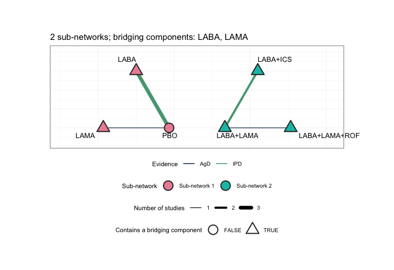

plot of chunk network-plot

plot() draws each sub-network on its own circle, so the disconnection is visible rather than inferred: the MONO-* trials sit around PBO on one circle, the ADD-* trials on the other, and no edge runs between them. Edge color separates the two IPD trials from the five aggregate ones, and node shape marks the treatments that contain a bridging component. Every treatment except PBO contains LABA or LAMA, which is precisely why the additive model has anything to bridge with; a network whose sub-networks shared no component could not be reconnected at all, and plot() would say so in its subtitle.

Two sub-networks, bridged by LABA and LAMA, and the component design matrix $X = BC$ has full column rank: an aggregate-data component NMA would identify every component effect and every relative effect (Rücker et al. 2020; Wigle et al. 2026). Hold that thought.

Covariate balance

balance <- do.call(rbind, lapply(split(patients, patients$.study), function(d)
  data.frame(Study = d$.study[1],
             Eosinophils = 200 + 100 * mean(d$eos),
             eos_mean = mean(d$eos), eos_sd = sd(d$eos),
             freqex = mean(d$freqex),
             Rate_per_year = sum(d$.y) / sum(d$.exposure))))
knitr::kable(balance, digits = 2, row.names = FALSE,
             caption = "Effect-modifier balance across the seven trials")

Effect-modifier balance across the seven trials
Study	Eosinophils	eos_mean	eos_sd	freqex	Rate_per_year
ADD-1	280.29	0.80	1.10	0.55	1.04
ADD-2	299.80	1.00	0.98	0.66	1.12
ADD-3	260.53	0.61	0.99	0.51	1.08
MONO-1	220.10	0.20	1.01	0.33	1.32
MONO-2	171.03	-0.29	0.90	0.29	1.08
MONO-3	206.57	0.07	1.01	0.41	1.38
MONO-4	238.85	0.39	1.01	0.48	1.37

The older MONO-* trials enrolled patients around 170-240 eosinophils, of whom roughly a third were frequent exacerbators. The newer ADD-* trials enrolled patients around 260-300 eosinophils, of whom more than half were. The two sub-networks are not comparing the same people, and both covariates move together, which is why the integration uses a copula rather than treating them as independent.

We must name a target population. Take the patients a formulary committee is actually deciding for: an eosinophilic, frequently exacerbating group (350 cells, 55% frequent exacerbators). We will also ask for a low-eosinophil, infrequently exacerbating population, where the answer is quite different.

target     <- data.frame(eos =  1.5, freqex = 0.55)   # 350 cells, 55% frequent
target_low <- data.frame(eos = -0.5, freqex = 0.20)   # 150 cells, 20% frequent

Fitting

Route 1: two stages, frequentist

cstc() regresses the count on treatment, the covariate main effects, and treatment-by-modifier interactions, with a log(exposure) offset and the modifiers centered at the target; its treatment coefficient is then the population-adjusted conditional log rate ratio in the target population. cmaic() reweights each IPD trial so its modifier distribution matches the target (Signorovitch et al. 2010) and refits a weighted Poisson model with the same offset, giving a marginal log rate ratio. Both hand their adjusted contrasts to cnma_bridge().

ems <- c("eos", "freqex")

fit_stc <- cstc(net, target = c(eos = 1.5, freqex = 0.55), effect_modifiers = ems)

fit_maic <- cmaic(net, target = c(eos = 1.5, freqex = 0.55),
                  target_sd = c(eos = 1.0),      # only the continuous one needs an SD
                  effect_modifiers = ems, n_boot = 200, seed = 9)
effective_sample_size(fit_maic)
#>   MONO-1    ADD-1 
#> 236.6135 823.9037

target_sd names only eos. A Bernoulli variable’s mean fixes its variance, so matching freqex’s prevalence already matches its second moment; there is nothing extra to ask for.

Matching costs information, and the effective sample sizes show how much. MONO-1 is the trial furthest from the target on both covariates, and it pays heavily: most of its patients receive very little weight, because the target population barely resembles them. That number is a warning, not a diagnostic to be optimized away; a small ESS means the adjusted contrast rests on a handful of patients (Phillippo et al. 2018).

An effective sample size says that the weights are well behaved. It does not say that the reweighted edge carries the contrast you care about, and if it does not, then adjusting that edge cannot move the answer however healthy its ESS looks. plot_edge_influence() asks the second question directly: it decomposes the bridged estimate of one contrast into the weight each observed edge receives.

plot_edge_influence(fit_stc, treatment = "LABA+ICS", comparator = "LAMA")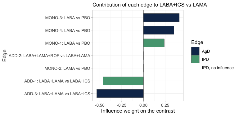

plot of chunk edge-influence

Both IPD edges carry weight, so the population adjustment done to them is not wasted. The reason is worth spelling out, because it is the whole logic of the bridge: LABA+ICS versus LAMA decomposes into the LABA direction, which MONO-1, MONO-3 and MONO-4 measure, plus the LAMA minus ICS direction, which ADD-1 and ADD-3 measure. MONO-1 and ADD-1 are the IPD trials, and they sit one in each of those directions.

Two edges get nothing. ADD-2 is the easy case: the headline contrast contains no ROF component, so the roflumilast trial is irrelevant to it. MONO-2 is the instructive one. It measures LAMA against PBO, so its edge points along LAMA alone, and that is not one of the two directions the contrast decomposes into; the bridge therefore takes nothing from it, despite its being the only trial in the network that studied LAMA on its own. Had either of those zero-weight edges been an IPD trial, it would have been drawn in red: reweighting an edge of no influence cannot change the answer, whatever its effective sample size reports.

The two-stage answer, as a forest plot, with LAMA as the comparator throughout:

forest(fit_stc, reference = "LAMA")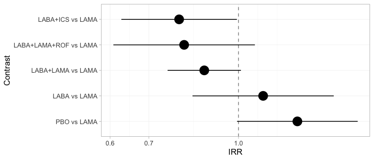

plot of chunk forest-freq

The bridge estimates all five contrasts against LAMA and flags none of them. That is not an oversight: the component design matrix has full column rank, so from the bridge’s point of view every relative effect is identified. Keep this figure in mind. The Bayesian forest in the Results section, fitted to the same seven trials, declines to report three of these five rows.

Two routes, two estimands

The two methods target different things, and we can check that directly. The adjusted contrast each hands to the bridge is stored on the fitted object, so we can line it up against the estimand it is supposed to be hitting: the true conditional log rate ratio in closed form, and the true marginal one by G-computation over the target population.

edge <- function(fitobj, study) {
  a <- fitobj$bridge$network$agd
  a$TE[a$studlab == study]
}
mu_of <- function(s) design$mu[design$study == s]

# true MARGINAL log rate ratio in the target population, by G-computation
mc_marginal <- function(mu, t1, t2, M = 3e5) {
  fx <- rbinom(M, 1, 0.55)
  x  <- cbind(eos = rnorm(M, 1.5, 1.0), freqex = fx)
  rate <- function(t) mean(exp(mu + as.vector(x %*% b_prog) +
    vapply(seq_len(M), function(i) theta(t, x[i, ]), numeric(1))))
  log(rate(t1)) - log(rate(t2))
}

x_tgt <- c(eos = 1.5, freqex = 0.55)
truth <- function(t1, t2, x) theta(t1, x) - theta(t2, x)

knitr::kable(data.frame(
  Edge = c("MONO-1: LABA vs PBO", "ADD-1: LABA+LAMA vs LABA+ICS"),
  true_conditional = c(truth("LABA", "PBO", x_tgt),
                       truth("LABA+LAMA", "LABA+ICS", x_tgt)),
  cSTC             = c(edge(fit_stc, "MONO-1"), edge(fit_stc, "ADD-1")),
  true_marginal    = c(mc_marginal(mu_of("MONO-1"), "LABA", "PBO"),
                       mc_marginal(mu_of("ADD-1"), "LABA+LAMA", "LABA+ICS")),
  cMAIC            = c(edge(fit_maic, "MONO-1"), edge(fit_maic, "ADD-1"))),
  digits = 3, row.names = FALSE,
  caption = "Adjusted log rate ratios handed to the bridge, against the estimand each targets")

Adjusted log rate ratios handed to the bridge, against the estimand each targets
Edge	true_conditional	cSTC	true_marginal	cMAIC
MONO-1: LABA vs PBO	-0.131	-0.181	-0.132	-0.274
ADD-1: LABA+LAMA vs LABA+ICS	0.260	0.254	0.249	0.203

Compare the true_conditional and true_marginal columns. They are almost the same number: on the MONO-1 edge they agree to three decimal places. That is collapsibility: on the rate-ratio scale, marginalizing over a covariate does not move the effect, and what little movement survives is the second-order Jensen term that exists only because $\Gamma \neq 0$ . Run the identical comparison on the odds-ratio scale (vignette("binary-outcomes")) and the two truths separate by about 10%. Same two functions, same network shape, different link: the estimand gap opens or closes according to the link, and nothing else.

So on a collapsible measure the cstc()-versus-cmaic() choice is not a choice of estimand, and you may pick on variance grounds instead. That is worth doing, and this table shows why: cmaic() is visibly the noisier of the two on the MONO-1 edge. Its effective sample size there collapsed to a few hundred of the 1200 patients, because MONO-1 is the trial furthest from the target, and the estimate pays for it. Regression adjustment uses every patient and is usually the more efficient. On a non-collapsible measure you do not get this luxury: there the choice is a choice of estimand, and it has to be made deliberately (Remiro-Azócar et al. 2022).

Route 2: one stage, Bayesian

fit <- cmlnmr(ipd, agd,
              effect_modifiers = ems,
              inactive = "PBO", family = "poisson",
              exposure = ".exposure",
              trt_effects = "random",
              chains = 4, iter_warmup = 500, iter_sampling = 500,
              n_int = 64, seed = 3, show_exceptions = FALSE)
fit
#> cpaic: component-additive ML-NMR (Bayesian, poisson)
#>   Treatment effects: random (noncentered)
#>   Effect modifiers: eos [normal], freqex [bernoulli]
#>   Component effects below are at the covariate origin (x = 0).
#>   For a target population use relative_effects(fit, newdata = ...).
#> 
#>  component estimate    se  lower upper
#>        ICS   -0.126 0.178 -0.450 0.192
#>       LABA   -0.133 0.099 -0.319 0.046
#>       LAMA   -0.122 0.148 -0.368 0.184
#>        ROF   -0.387 1.061 -2.848 1.181

The [bernoulli] and [normal] tags in the print output are the integration margins cpaic chose. It guessed them from the IPD (freqex is 0/1, eos is not); margins = c(freqex = "bernoulli", eos = "normal") would set them explicitly.

Priors

knitr::kable(do.call(rbind, lapply(names(fit$priors), function(p) {
  s <- fit$priors[[p]]
  data.frame(parameter = p, distribution = s$distribution,
             location = s$location, scale = s$scale)
})), caption = "The complete prior specification, as passed to Stan")

The complete prior specification, as passed to Stan
parameter	distribution	scale
intercept	normal	2.5
beta	normal	2.5
regression	normal	1.0
gamma	normal	1.0
tau	half-normal	1.0

The interaction prior, normal(0, 1), deserves a second look on this scale. Exacerbation log rate ratios are small numbers: the component main effects here are all between $-0.25$ and $-0.12$ . A normal(0, 1) prior on an interaction is therefore very permissive relative to the effects we are estimating, and it does real regularizing work only where $\Gamma$ is weakly identified. That is exactly where we will need prior_sensitivity() below.

plot_prior_posterior() shows the same thing without a refit, overlaying each parameter’s posterior (histogram) on the prior it was given (red line). A posterior that reproduces its prior was not estimated from the data.

plot_prior_posterior(fit)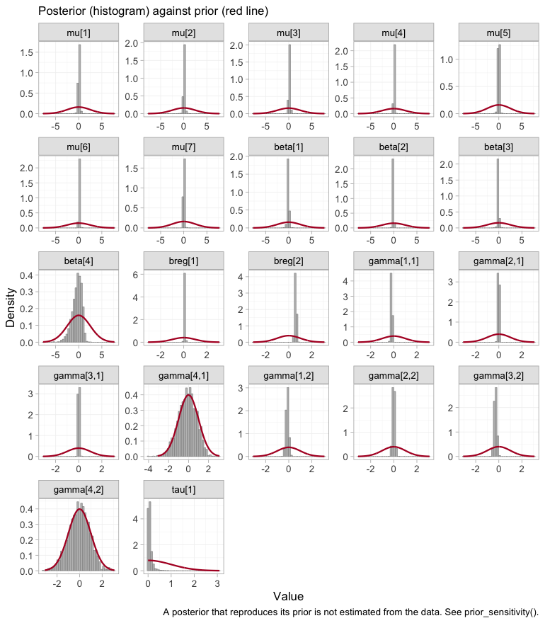

plot of chunk prior-posterior

The seven study intercepts mu and the two prognostic coefficients breg are spikes against a broad prior: the likelihood moved them, and hard. Three of the four component main effects beta do the same. The interactions gamma split into two groups, and the indexing is what makes the panels readable: the first index runs over the components in the order ICS, LABA, LAMA, ROF, the second over the modifiers eos and freqex. Six of the eight interactions are pulled well inside their prior. The two that are not, gamma[4,1] and gamma[4,2], sit squarely on top of the red curve, and the one beta that barely moved is beta[4]. All three belong to roflumilast. We return to them under prior sensitivity, and they will turn up again, uninvited, in the integration diagnostics below.

Convergence

data.frame(
  divergences   = fit$diagnostics$divergences,
  max_treedepth = fit$diagnostics$max_treedepth,
  max_rhat      = round(fit$diagnostics$max_rhat, 4),
  min_ess_bulk  = round(min(fit$fit$summary(c("beta", "gamma", "mu",
                                              "tau"))$ess_bulk, na.rm = TRUE))
)
#>   divergences max_treedepth max_rhat min_ess_bulk
#> 1           4             1   1.0085          396

No divergences, and $\hat R$ and the effective sample sizes are fine. A handful of iterations saturate the maximum tree depth, which costs efficiency rather than correctness; it is the signature of the mild funnel that any random-effects model has when tau is only weakly informed. Raising max_treedepth (passed through ... to cmdstanr) removes it at the cost of runtime.

The same conclusion, drawn rather than tabulated. plot() on a cmlnmr() fit hands the draws to bayesplot; type = "trace" shows the four chains for the component effects, the interactions, and the heterogeneity.

plot(fit, type = "trace")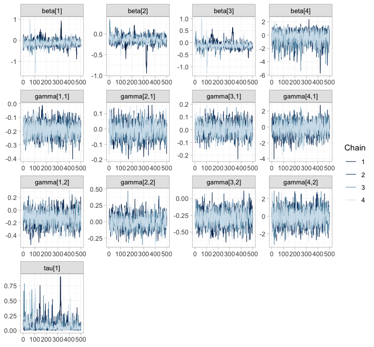

plot of chunk trace

plot(fit, type = "rhat")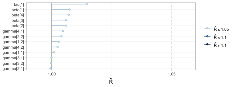

plot of chunk rhat

The chains overlay one another and sweep the whole support of each parameter, with no drift and no chain exploring a region of its own; every $\hat R$ sits in the lowest band. Now notice what these two figures cannot tell you. Compare the gamma[4, ] panels, which range across roughly plus or minus 3, with gamma[2, ], which barely leave a tenth of that. The wide pair belongs to roflumilast, whose interactions no trial in this network identifies; the narrow pair belongs to LABA, which two IPD arms pin down. Both mix beautifully. Sampling from a prior is easy, and a sampler has no way of minding that it is doing so. Convergence diagnostics certify that the posterior was explored; they say nothing whatever about whether it was informed, and the rest of this vignette is about the difference.

Integration accuracy

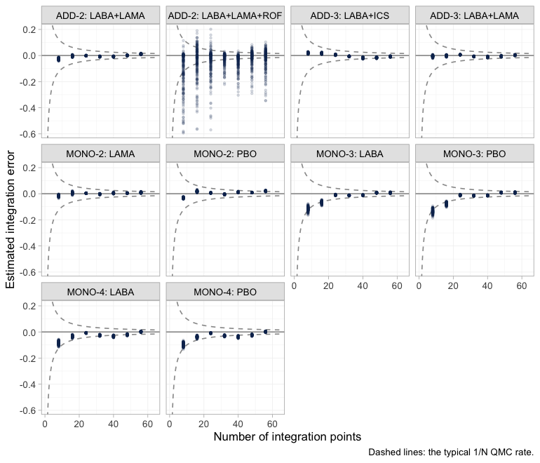
The aggregate likelihood is a quasi-Monte-Carlo integral, so it carries a numerical error on top of the statistical one. plot_integration_error() traces it: for each aggregate arm it recomputes the integrated rate from the first $N$ integration points, subtracts the value at all 64, and compares the residual against the $1/N$ envelope that quasi-Monte-Carlo integration is expected to follow.

plot_integration_error(fit)

plot of chunk integration-error

Nine of the ten aggregate arms behave as they should: the error collapses onto zero well inside the envelope, long before 64 points. The tenth does not, and it is worth knowing which one. ADD-2’s LABA+LAMA+ROF arm has an error an order of magnitude larger than any other arm’s, still smeared across the envelope at the right-hand edge.

More integration points would not fix it, because the spread is not really across integration points: it is across posterior draws. Roflumilast’s interactions are the ones no trial identifies, and their posterior therefore runs over the whole prior, as the prior-versus-posterior figure above already showed. A draw with a large gamma[4, ] makes the integrand $\exp(x^\top(b + \Gamma^\top C_k))$ vary enormously across the covariate distribution, and any Monte-Carlo average of a wildly varying integrand converges slowly. The control is sitting right beside it: ADD-2’s other arm, LABA+LAMA, integrates perfectly cleanly. Same trial, same patients, same covariate distribution, same 64 points. The only difference between the two arms is the ROF component.

So the numerical diagnostic has independently fingered the same component the estimability algebra refuses to report, and that is the lesson worth carrying away: a badly behaved integration facet is sometimes a symptom of a badly identified parameter rather than of too few integration points. Nothing here contaminates the results, because every contrast involving ROF is returned as NA in any case. Had a facet misbehaved on an arm whose contrasts we do report, the remedy would be to refit with a larger n_int before reading the estimates.

Estimability: more effect modifiers, fewer estimable effects

Here is the count-specific twist, and it is not intuitive.

An aggregate two-arm trial contributes one number per contrast: it pins down $m^\top(\beta + \Gamma \bar x_j)$ at its own covariate mean $\bar x_j$ , and no more. But the population-adjusted estimand $m^\top(\beta + \Gamma x)$ has $1 + Q$ unknowns in the direction $m$ : one main effect and $Q$ interactions. So an aggregate-only component needs $1 + Q$ independent aggregate equations to be identified at a general target.

With one effect modifier that is two equations. With two effect modifiers it is three. Adding a modifier to the model makes the aggregate-only components strictly harder to identify, even though it makes the model more nearly correct. An IPD trial escapes this, because within a trial you can regress on arm and on arm-by-covariate directly, and so recover all $1 + Q$ at once.

estimable_effects_at(fit, newdata = target, reference = "LAMA")
#> Estimability of the population-adjusted relative effects
#>   Target population: eos = 1.5, freqex = 0.55
#>      treatment comparator estimable identified_by          basis
#>           LABA       LAMA     FALSE          none not identified
#>       LABA+ICS       LAMA      TRUE           IPD          exact
#>      LABA+LAMA       LAMA      TRUE           IPD          exact
#>  LABA+LAMA+ROF       LAMA     FALSE          none not identified
#>            PBO       LAMA     FALSE          none not identified
#> 
#>   Rows marked "not identified" carry no first-order information; a number
#>   reported for them would be the prior. relative_effects() returns NA there.

LABA+ICS (the headline) and LABA+LAMA are identified, from IPD. The other three are not identified at all, because each needs LAMA or ROF on its own, and each of those is seen in exactly one aggregate contrast: one equation, three unknowns.

Estimability depends on the target. MONO-2 is the aggregate trial that measured LAMA; ask for its population and LAMA comes back:

mono2 <- agd[agd$.study == "MONO-2", ]
own   <- data.frame(eos = mean(mono2$eos_mean), freqex = mean(mono2$freqex_mean))
own
#>          eos    freqex
#> 1 -0.2896867 0.2908333
estimable_effects_at(fit, newdata = own, reference = "LAMA")
#> Estimability of the population-adjusted relative effects
#>   Target population: eos = -0.29, freqex = 0.291
#>      treatment comparator estimable identified_by              basis
#>           LABA       LAMA      TRUE     aggregate first-order screen
#>       LABA+ICS       LAMA      TRUE           IPD              exact
#>      LABA+LAMA       LAMA      TRUE           IPD              exact
#>  LABA+LAMA+ROF       LAMA     FALSE          none     not identified
#>            PBO       LAMA      TRUE     aggregate first-order screen
#> 
#>   Rows marked "first-order screen" are estimable by the linear criterion, which
#>   is only a design-based screen for them (aggregate identification, or a
#>   survival baseline) and can be optimistic. Check them with prior_sensitivity().
#> 
#>   Rows marked "not identified" carry no first-order information; a number
#>   reported for them would be the prior. relative_effects() returns NA there.

That is the whole of what an aggregate two-arm trial can tell you: its own contrast, in its own population. Everything else is extrapolation through $\Gamma$ , and $\Gamma$ has to come from somewhere.

plot_estimability() makes that statement into a picture. It sweeps the target population along one effect modifier and re-asks the estimability question at every point. We sweep eos through a grid that passes exactly through MONO-2’s own eosinophil mean, holding freqex at MONO-2’s own prevalence, so that one column of the map, and only one, is MONO-2’s own population.

eos_grid <- own$eos + seq(-1, 3, by = 0.5)
plot_estimability(fit, em = "eos", values = eos_grid,
                  at = c(freqex = own$freqex), reference = "LAMA") +
  theme(plot.caption = element_text(size = 6.5))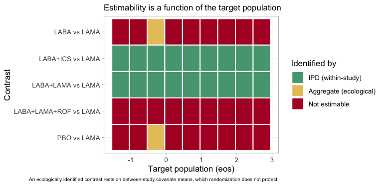

plot of chunk estimability-map

Three colors, three regimes. Two rows are green across the entire axis: the headline contrast LABA+ICS versus LAMA, and LABA+LAMA versus LAMA. Both are identified by IPD, from within-study arm-by-covariate variation, and are therefore identified in every target population; that within-study variation is exactly what anchored STC and MAIC consume. Two more rows, PBO versus LAMA and LABA versus LAMA, are red everywhere except at the single column that is MONO-2’s own population, where they turn yellow. There, and nowhere else, the aggregate LAMA trial identifies its own contrast, and anything that can be built from it; and it does so ecologically, from a between-study covariate mean rather than from a within-study slope (Berlin et al. 2002). The roflumilast row is red throughout, because ADD-2’s own population does not lie on this axis. A one-column island of estimability is what an aggregate two-arm trial buys you.

The same algebra reaches the component effects:

component_effects(fit, newdata = target)
#>   component   estimate        se      lower      upper
#> 1       ICS         NA        NA         NA         NA
#> 2      LABA -0.1474449 0.1058796 -0.3378115 0.03994639
#> 3      LAMA         NA        NA         NA         NA
#> 4       ROF         NA        NA         NA         NA

LABA is identified. ICS, LAMA and ROF individually are not; but the combination the headline needs, LABA plus ICS minus LAMA, is, because ADD-1 measured LAMA against ICS with IPD. cpaic returns NA for what it cannot identify rather than a prior-driven number, which is the behavior you want from a tool that would otherwise hand you the prior with a straight face (Wigle et al. 2026).

forest(fit, what = "component", newdata = target)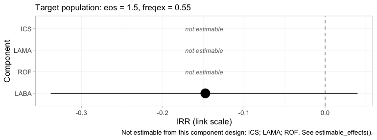

plot of chunk comp-forest

The component forest reports the same four numbers, on the log rate-ratio scale, and it keeps the three it cannot compute, drawn as labelled empty rows rather than dropped. A reader shown only LABA would have no way of telling that three components had been quietly removed; a reader shown three blanks knows exactly what the network could not answer.

Results

Recovered against the truth

relative_effects(fit, reference = "LAMA", newdata = target)
#> Relative effects (IRR, back-transformed)
#>   Target population: eos = 1.5, freqex = 0.55
#>      treatment comparator estimate    se lower upper pr_gt0
#>           LABA       LAMA       NA    NA    NA    NA     NA
#>       LABA+ICS       LAMA    0.711 0.154 0.528 0.911  0.009
#>      LABA+LAMA       LAMA    0.868 0.106 0.713 1.041  0.054
#>  LABA+LAMA+ROF       LAMA       NA    NA    NA    NA     NA
#>            PBO       LAMA       NA    NA    NA    NA     NA
#>   NA = not uniquely estimable from this component design (see estimable_effects()).

forest(fit, newdata = target, reference = "LAMA") +
  theme(plot.caption = element_text(size = 6.5))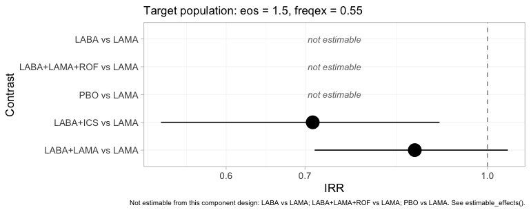

plot of chunk forest-bayes

The same table as a figure, and the refusals are now impossible to miss: PBO, LABA and LABA+LAMA+ROF versus LAMA are drawn as labelled empty rows. Set this beside the frequentist forest from the previous section, which put a point estimate and a confidence interval on all five. Same seven trials, same additive component structure, same target population. The difference is that one model knows which of its own answers this target identifies and the other does not.

relative_effects(fit, reference = "LAMA", newdata = target_low)
#> Relative effects (IRR, back-transformed)
#>   Target population: eos = -0.5, freqex = 0.2
#>      treatment comparator estimate    se lower upper pr_gt0
#>           LABA       LAMA       NA    NA    NA    NA     NA
#>       LABA+ICS       LAMA    1.009 0.158 0.728 1.318  0.505
#>      LABA+LAMA       LAMA    0.882 0.097 0.731 1.050  0.064
#>  LABA+LAMA+ROF       LAMA       NA    NA    NA    NA     NA
#>            PBO       LAMA       NA    NA    NA    NA     NA
#>   NA = not uniquely estimable from this component design (see estimable_effects()).

The headline rate ratio moves from roughly 0.7 in the eosinophilic target to roughly 0.9 in the low-eosinophil one: the steroid earns its place in one population and barely in the other. Now put every method beside the planted truth.

grab <- function(tab, t1, ref, what = "estimate") {
  as.numeric(tab[[what]][tab$treatment == t1 & tab$comparator == ref])
}
re_bayes <- relative_effects(fit, reference = "LAMA", newdata = target)
re_stc   <- relative_effects(fit_stc,  reference = "LAMA")
re_maic  <- relative_effects(fit_maic, reference = "LAMA")

ci <- function(tab, t1) sprintf("(%.2f, %.2f)", grab(tab, t1, "LAMA", "lower"),
                                                grab(tab, t1, "LAMA", "upper"))
covers <- function(tab, t1) {
  tr <- exp(truth(t1, "LAMA", x_tgt))
  ifelse(tr >= grab(tab, t1, "LAMA", "lower") &&
         tr <= grab(tab, t1, "LAMA", "upper"), "yes", "NO")
}
recovery <- do.call(rbind, lapply(c("LABA+ICS", "LABA+LAMA"), function(t1) {
  data.frame(
    Contrast    = paste(t1, "vs LAMA"),
    True_RR     = exp(truth(t1, "LAMA", x_tgt)),
    cSTC        = grab(re_stc,  t1, "LAMA"),
    `cSTC covers` = covers(re_stc, t1),
    cMAIC       = grab(re_maic, t1, "LAMA"),
    `cML-NMR`   = grab(re_bayes, t1, "LAMA"),
    `cML-NMR 95% CrI` = ci(re_bayes, t1),
    `cML-NMR covers`  = covers(re_bayes, t1),
    check.names = FALSE)
}))
knitr::kable(recovery, digits = 3, row.names = FALSE,
  caption = "Rate ratios in the target population, against the truth")

Rate ratios in the target population, against the truth
Contrast	True_RR	cSTC	cSTC covers	cMAIC	cML-NMR	cML-NMR 95% CrI	cML-NMR covers
LABA+ICS vs LAMA	0.676	0.790	yes	0.803	0.711	(0.53, 0.91)	yes
LABA+LAMA vs LAMA	0.877	0.873	yes	0.870	0.868	(0.71, 1.04)	yes

Three things to notice.

First, cstc() and cmaic() land on essentially the same number, as the estimand table above predicted they would: on a collapsible scale the two estimands nearly coincide.

Second, cmlnmr() sits closer to the truth than either of them on the headline contrast. That is not luck. The ADD-3 trial measured the same comparison as our IPD trial ADD-1, but it is aggregate, so cstc() and cmaic() cannot adjust it: it enters cnma_bridge() at its own eosinophil level (around 260 cells), and ICS is strongly eosinophil-modified, so it drags the pooled estimate toward the weaker effect that held in its population. cmlnmr() has no such problem, because it integrates every aggregate arm over that arm’s own covariate distribution inside the likelihood. The two-stage route is biased even on contrasts that are formally estimable, in proportion to how much unadjusted aggregate evidence sits on the same edge.

Third, the credible interval covers the truth. So, here, does the confidence interval; but it is aimed slightly off, and in a network with more aggregate evidence on that edge it would miss.

The whole set of pairwise answers, for completeness:

knitr::kable(league_table(fit, newdata = target),
  caption = paste("League table in the target population: rate ratio of the row",
                  "treatment versus the column treatment, with its 95% credible",
                  "interval. Blank cells are not identified at this target."))

League table in the target population: rate ratio of the row treatment versus the column treatment, with its 95% credible interval. Blank cells are not identified at this target.
	LABA	LABA+ICS	LABA+LAMA	LABA+LAMA+ROF	LAMA	PBO
LABA	LABA					0.87 (0.71, 1.04)
LABA+ICS		LABA+ICS	0.82 (0.66, 0.98)		0.71 (0.53, 0.91)
LABA+LAMA		1.23 (1.02, 1.51)	LABA+LAMA		0.87 (0.71, 1.04)
LABA+LAMA+ROF				LABA+LAMA+ROF
LAMA		1.44 (1.10, 1.89)	1.17 (0.96, 1.40)		LAMA
PBO	1.17 (0.96, 1.40)					PBO

A league table with holes in it. Only two blocks of cells carry numbers: PBO against LABA, and the three-way block among LAMA, LABA+ICS and LABA+LAMA. Every blank cell is one whose contrast would need the effect of LAMA, or of ROF, on its own, and neither is pinned down at this target. LABA+LAMA+ROF has an entirely empty row and an entirely empty column: no other treatment in the network differs from it by a set of components the design can resolve here. A conventional league table would have printed all thirty numbers and told the reader nothing about which twenty-two of them the design cannot identify at this target.

grid <- seq(-1, 3, by = 0.2)
curve <- do.call(rbind, lapply(grid, function(e) {
  re <- relative_effects(fit, reference = "LAMA",
                         newdata = data.frame(eos = e, freqex = 0.55))
  r <- re[re$treatment == "LABA+ICS", ]
  data.frame(eos = e, est = r$estimate, lo = r$lower, hi = r$upper,
             truth = exp(truth("LABA+ICS", "LAMA", c(eos = e, freqex = 0.55))))
}))
ggplot(curve, aes(200 + 100 * eos)) +
  geom_ribbon(aes(ymin = lo, ymax = hi), alpha = 0.15) +
  geom_line(aes(y = est, color = "cML-NMR posterior mean"), linewidth = 1) +
  geom_line(aes(y = truth, color = "Truth"), linetype = "dashed",
            linewidth = 1) +
  geom_hline(yintercept = 1, color = "grey50") +
  scale_y_log10() +
  scale_color_manual(values = c("cML-NMR posterior mean" = "#2c7fb8",
                                 "Truth" = "#d95f0e")) +
  labs(x = expression("Blood eosinophils in the target population (cells /" ~ mu * "L)"),
       y = "Rate ratio, LABA+ICS vs LAMA (log scale)", color = NULL,
       title = "The steroid earns its place only in eosinophilic patients",
       subtitle = "Frequent-exacerbator prevalence held at 55%; the contrast no trial measured") +
  theme_minimal() + theme(legend.position = "top")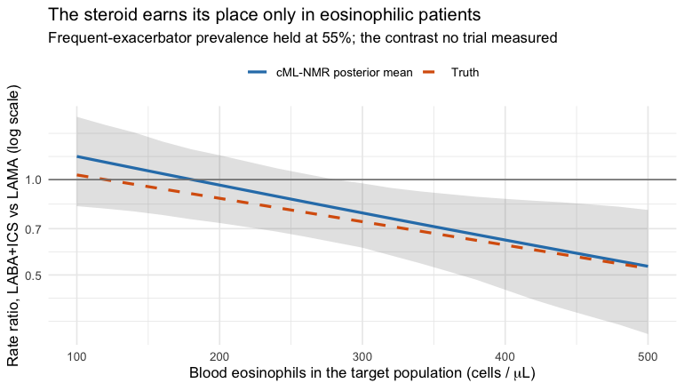

plot of chunk pop-curve

What the frequentist bridge does with the effects it cannot identify

cstc() and cmaic() adjust only the edges where you hold IPD. Every aggregate edge enters cnma_bridge() in its own trial’s population, and the additive model then propagates that into any contrast that leans on it, with no warning. Look at the contrasts cmlnmr() refused to report:

cmp <- do.call(rbind, lapply(c("PBO", "LABA", "LABA+LAMA+ROF"), function(t1) {
  data.frame(
    Contrast  = paste(t1, "vs LAMA"),
    True_RR   = exp(truth(t1, "LAMA", x_tgt)),
    cSTC      = grab(re_stc,   t1, "LAMA"),
    cMAIC     = grab(re_maic,  t1, "LAMA"),
    `cML-NMR` = grab(re_bayes, t1, "LAMA"),
    check.names = FALSE)
}))
knitr::kable(cmp, digits = 3, row.names = FALSE,
  caption = "Rate ratios cML-NMR declines to report, and what the bridge prints anyway")

Rate ratios cML-NMR declines to report, and what the bridge prints anyway
Contrast	True_RR	cSTC	cMAIC	cML-NMR
PBO vs LAMA	1.370	1.264	1.264	NA
LABA vs LAMA	1.202	1.103	1.099	NA
LABA+LAMA+ROF vs LAMA	0.757	0.805	0.803	NA

The frequentist bridge prints a confident number for each of these, and here those numbers are not far off. That is worth being honest about, and it is worth understanding, because it is luck rather than method: in this network the aggregate-only components happen to be weakly effect-modified in the directions that matter (Gamma_true["LAMA", "eos"] = 0.01, and roflumilast barely interacts with anything), so evaluating their contrasts in the wrong population costs little.

Change Gamma_true["LAMA", "eos"] to something substantial and those cells would be badly wrong, with intervals that exclude the truth; that is exactly what happens in vignette("binary-outcomes"), where the aggregate-only component is strongly effect-modified. You cannot know which case you are in without fitting a model that can tell you. The NA is not the tool being unhelpful; it is the tool declining to pretend.

The hierarchy the network can support

Everyone wants the ranking. Wigle et al. (2026) set out a four-step workflow for producing one honestly, and its third step is the one that bites here: refine the ranked set to the elements that are actually estimable, or decline to rank. cpaic performs that refinement automatically. Because the outcome is a rate of exacerbations, fewer is better, so every ranking call below is passed lower_is_better = TRUE.

plot(cpaic_ranks(fit, newdata = target, lower_is_better = TRUE))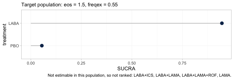

plot of chunk ranks-target

Step 3 is drastic in this network. Four of the six treatments leave the hierarchy, and the caption names them. What survives is a two-element comparison between placebo and LABA, which is not a question anybody asked. The alternative was to rank all six, in which case four of the six ranks would have been functions of the interaction prior rather than of any trial, and the figure would have looked complete.

The rankogram is stricter still, and it is worth seeing it refuse:

tryCatch(
  plot(rank_probs(fit, newdata = target, lower_is_better = TRUE)),
  error = function(e) cat(strwrap(conditionMessage(e), 76), sep = "\n"))
#> Fewer than two elements are estimable in this target population, so no
#> hierarchy can be formed. See estimable_effects_at().

rank_probs() ranks the treatments other than the reference, so, unlike cpaic_ranks(), it has no placebo to fall back on; after Step 3 only LABA remains, and one element is not a hierarchy. It therefore stops rather than draw one. That refusal is the intended behavior and not a defect: a rankogram computed from a prior-driven posterior is a picture of the prior, and it is indistinguishable, to the eye, from a picture of evidence.

Move the target to MONO-2’s own population, the one place on the eosinophil axis where the aggregate LAMA evidence bites, and the hierarchy returns:

plot(rank_probs(fit, newdata = own, lower_is_better = TRUE))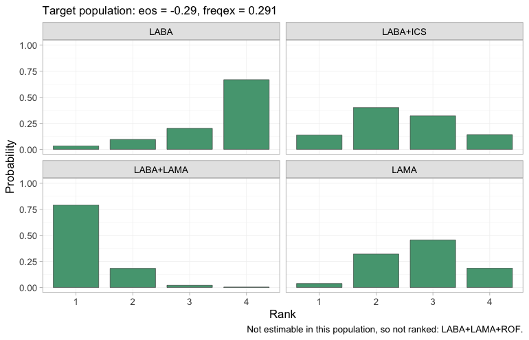

plot of chunk rankogram-own

Four treatments are now estimable and therefore ranked, each panel giving the posterior probability that the treatment takes each rank, with rank 1 the fewest exacerbations. The dual bronchodilator LABA+LAMA takes first place with high probability, and LABA alone is most likely to come last, which is what one would expect of the weakest active regimen in a low-eosinophil population where the steroid has little to offer. LABA+LAMA+ROF is still absent, because nothing identifies roflumilast in this population either. The point is not that MONO-2’s population is a better one to decide in; it is that the hierarchy, exactly like the estimable set and the relative effects themselves, is a property of the target population and not of the network.

The rank curve is designed to show that dependence directly, tracing each element’s SUCRA as the target moves:

plot_rank_curve(fit, em = "eos", values = seq(-1, 3, by = 0.5),
                at = c(freqex = 0.55), lower_is_better = TRUE) +
  theme(plot.subtitle = element_text(size = 7.5))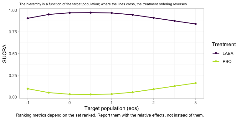

plot of chunk rank-curve

Two lines, a wide gap apart, that never come close to crossing, and it would be a serious misreading to take that as reassurance. The plot’s own subtitle offers to show you where the ordering reverses, and nothing reverses; but the reason is not that the hierarchy is stable. It is that at every target on this axis Step 3 leaves the same two-element set, placebo and LABA, and a two-element hierarchy contains nothing that could cross. What the curve actually traces is the posterior probability that LABA beats placebo. A rank curve that refuses to move means something only once the estimability map beside it has confirmed that there was more than one thing there to move. The figure this one is failing to be is a set of curves that cross; the failure is a property of the evidence, not of the plot.

Random effects and model comparison

tau is the study-arm heterogeneity around the component-implied effects. With seven contrasts and four components there are three degrees of freedom for it, so it is informed, but not richly.

knitr::kable(fit$fit$summary("tau")[, c("variable", "mean", "sd", "q5", "q95",
                                        "rhat", "ess_bulk")], digits = 3)

variable	mean	sd	q5	q95	rhat	ess_bulk
tau[1]	0.082	0.094	0.006	0.25	1.015	396.395

Compare against a fixed-effect fit by leave-one-out cross-validation (Vehtari et al. 2017) and DIC (Spiegelhalter et al. 2002):

fit_fixed <- cmlnmr(ipd, agd, effect_modifiers = ems, inactive = "PBO",
                    family = "poisson", exposure = ".exposure",
                    trt_effects = "fixed",
                    chains = 4, iter_warmup = 500, iter_sampling = 500,
                    n_int = 64, seed = 3, show_exceptions = FALSE)

loo::loo_compare(list(random = loo::loo(fit), fixed = loo::loo(fit_fixed)))
#>   model elpd_diff se_diff p_worse       diag_diff      diag_elpd
#>   fixed       0.0     0.0      NA                 4 k_psis > 0.7
#>  random      -1.1     0.7    0.94 |elpd_diff| < 4 8 k_psis > 0.7

knitr::kable(data.frame(
  model = c("random", "fixed"),
  DIC   = c(dic(fit)$dic, dic(fit_fixed)$dic),
  p_eff = c(dic(fit)$p_eff, dic(fit_fixed)$p_eff)),
  digits = 1, caption = "Deviance information criterion")

Deviance information criterion
model	DIC	p_eff
random	6244.1	20.4
fixed	6241.0	17.3

Two cautions on the LOO comparison. First, its Pareto- $k$ diagnostic flags several observations, and it is right to: each aggregate arm is a single “observation” carrying an entire trial’s worth of information, so leaving one out is a large perturbation and the importance-sampling approximation strains. Read LOO here as indicative, alongside DIC. Second, neither criterion tests the assumption that bridges the gap.

Two dic() objects passed to plot() give the dev-dev plot, which compares the models point by point instead of in aggregate:

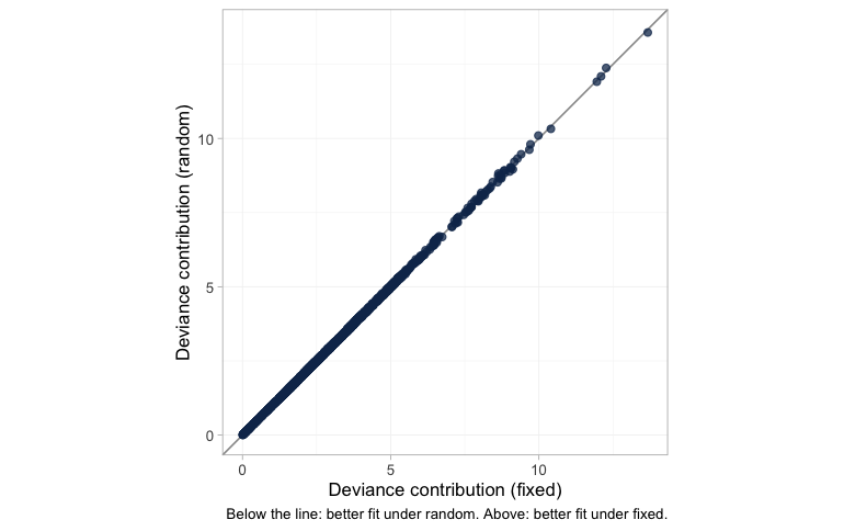
plot(dic(fit_fixed), dic(fit), labels = c("fixed", "random"))

plot of chunk devdev

Each dot is one data point’s posterior mean deviance under the fixed-effect model against its deviance under the random-effects model; below the line of equality the random-effects model fits it better, above it the fixed-effect model does. Nothing is below the line and nothing is above it. All 2410 points, the 2400 individual patients in the dense lower-left mass and the 10 aggregate arms trailing out to the upper right, are fitted identically by the two models. That is the DIC and LOO comparison drawn point by point rather than summed: tau is small enough that permitting study-arm heterogeneity changes no individual fit, which is why neither criterion can separate the models and why the choice between them here has to be made on grounds other than fit.

plot_leverage() asks which data points are buying that fit, plotting each point’s leverage (its contribution to the effective number of parameters) against its signed square root residual deviance, with contours of constant DIC contribution:

plot_leverage(fit)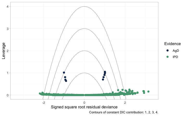

plot of chunk leverage

An individual patient carries almost no leverage, so the IPD lie in a flat band along the bottom. Their residual deviances fan out to either side, and a few sit beyond the outermost contour; that is expected rather than alarming, because a single Poisson count has irreducible deviance and no model fits one patient exactly. The contours are calibrated for arm-level points, and there the reading is clean: the aggregate arms sit an order of magnitude higher, at a leverage near one apiece, each being an entire trial compressed into a single count, and every one of them falls inside the DIC = 3 contour. No aggregate arm is spoiling the fit. (This plot needs a saturated model to measure residual deviance against. Poisson counts have one; censored survival times do not, which is why a survival model cannot be given a leverage plot at all.)

The frequentist bridge offers a Cochran $Q$ . Read Q.diff, not Q: only the former tests the additivity restrictions, and on a disconnected network it does not exist at all, because there is no standard NMA to nest the additive model inside.

additivity_test(fit_stc)
#> Additive component model: fit statistics
#>   Total lack of fit (Q.additive): Q = 9.772, df = 3, p = 0.0206
#>   Additivity restrictions (Q.diff): not available; no standard NMA
#>     is estimable on a disconnected network.
#>   Note: neither statistic tests whether component effects are constant
#>   ACROSS sub-networks, which is the assumption that bridges the gap.
#>   That assumption is untestable from the data and must be justified
#>   clinically.

The total lack of fit Q.additive is nevertheless large here. Because we planted the truth, we know exactly why, and it is not a failure of additivity: the additive model is exactly right by construction. It is that the contrasts being pooled are not all in the same population. The aggregate edges enter at their own covariate means, the adjusted IPD edges at the target, the components are effect-modified, and so no single vector of component effects can fit them all. $Q$ is picking up the population heterogeneity that the two-stage route is ignoring. It cannot tell you that is the cause, but when you see it, this is a possibility to rule in or out before you blame additivity.

Prior sensitivity

A contrast that moves when you change a prior it should not depend on was never data-driven. prior_sensitivity() refits under a tighter and a looser interaction prior. It deliberately reports movement for the non-estimable contrasts too, bypassing the NA mask, so that you can see the mechanism instead of taking it on trust.

ps <- prior_sensitivity(fit, newdata = target, reference = "LAMA",
                        prior = "gamma", tighter = 0.5, looser = 2,
                        chains = 2, iter_warmup = 250, iter_sampling = 250)
ps
#> cML-NMR prior sensitivity: gamma prior
#>      treatment comparator estimate tighter looser move_tighter move_looser max_movement estimable
#>           LABA       LAMA    0.130   0.120  0.152        0.010       0.023        0.023     FALSE
#>       LABA+ICS       LAMA   -0.353  -0.328 -0.335        0.025       0.018        0.025      TRUE
#>      LABA+LAMA       LAMA   -0.147  -0.138 -0.141        0.010       0.007        0.010      TRUE
#>  LABA+LAMA+ROF       LAMA   -0.742  -0.380 -1.967        0.362       1.225        1.225     FALSE
#>            PBO       LAMA    0.277   0.258  0.293        0.020       0.016        0.020     FALSE

Read max_movement against estimable. The estimable contrasts barely move. The non-estimable ones move with the prior, and LABA+LAMA+ROF moves enormously: doubling the interaction prior’s scale swings its posterior mean by more than a log unit, because roflumilast’s interactions are informed by nothing except that prior. That is what “not identified” means. No likelihood ridge holds it in place, and yet the posterior looks perfectly healthy while the prior fills the vacuum.

plot_prior_posterior(fit, prior = "gamma") reaches the same verdict for the cost of no refit at all, by overlaying each interaction’s posterior on the normal(0, 1) prior it was handed:

plot_prior_posterior(fit, prior = "gamma")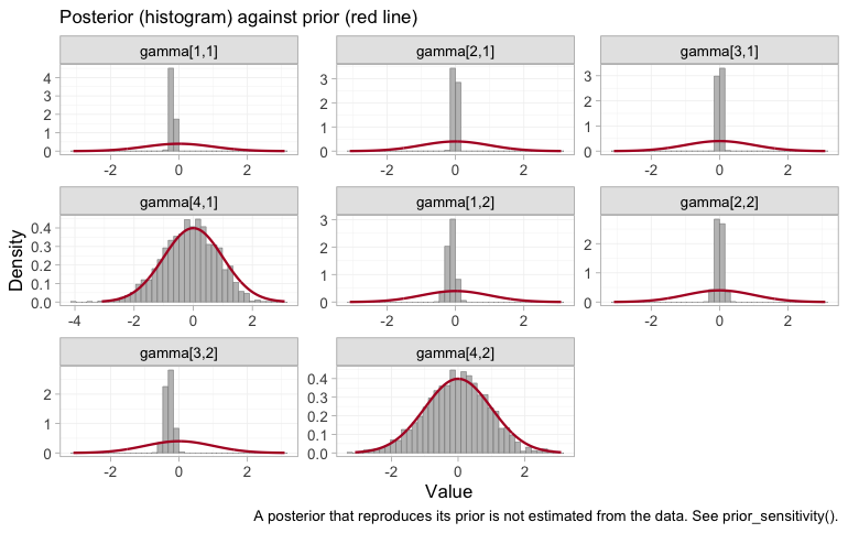

plot of chunk prior-posterior-gamma

Recall the indexing: components in the order ICS, LABA, LAMA, ROF, modifiers in the order eos, freqex. Two panels are unlike the rest, and they are gamma[4,1] and gamma[4,2]: roflumilast’s interactions with each modifier reproduce the normal(0, 1) prior almost exactly. Nothing in seven trials touched them, which is why doubling that prior’s scale swings LABA+LAMA+ROF by more than a log unit in the table above. A well-mixed chain sampling a prior is still sampling a prior, and no convergence diagnostic will ever say otherwise.

The other six interactions are pulled well inside their prior, and that deserves a word, because it is not the same statement as “estimable”. ICS and LAMA have tightly determined interactions here, and cpaic still reports their contrasts as NA. The two are consistent. Each of those components appears in an arm of an IPD trial, so the within-arm covariate slopes do constrain it, but only by borrowing the prognostic surface breg from MONO-1 to interpret ADD-1, which is to say only by assuming that the prognostic effects are the same in both trials. The criterion behind estimable_effects_at() is built from within-study arm contrasts, in which that surface cancels, so it never leans on the assumption and never claims the identification it would buy. The two diagnostics ask different questions: plot_prior_posterior() asks what the likelihood touched, and estimable_effects_at() asks what the design proves without extra assumptions. Roflumilast fails both. ICS and LAMA fail only the second, and it is on the strength of that failure, not of a wide posterior, that they are returned as NA.

Notice that this is true even though those same contrasts came out fairly close to the truth in the table above. Being right by luck and being identified are different properties, and only one of them is a reason to believe a number.

What to take away

	Adjusts the population	Bridges the gap	Reports non-identified effects
Standard NMA	no	no	not at all; they lie outside the model
ML-NMR	yes	no	yes, as prior-driven numbers
`cstc()` / `cmaic()` + `cnma_bridge()`	IPD edges only	yes	yes, silently
`cmlnmr()`	yes, all edges	yes	no: returns `NA`

Rates need an offset, and the log link needs integration. Person-time enters as log(exposure); the aggregate likelihood is the individual model averaged over the study’s covariate distribution on the rate scale, never evaluated at the covariate mean.
Collapsibility is a property of the link. On the rate-ratio scale cstc() and cmaic() target nearly the same thing and land nearly together. On the odds-ratio scale they do not. Do not carry an intuition from one to the other.
More effect modifiers means fewer estimable effects, for aggregate-only components. Each aggregate two-arm trial gives one equation; the estimand has $1 + Q$ unknowns per contrast direction. IPD is what breaks the tie, which is the whole reason population adjustment needs it.

Three honest limitations.

The bridging assumption is untestable. Reconnecting through shared components requires the component effects and their interactions with the effect modifiers to be equal in both sub-networks. There is, by construction, no cross-gap evidence with which to test that: neither Q, nor Q.diff, nor LOO can see it. It must be defended clinically (Veroniki et al. 2026).
A component effect identified only by aggregate data is identified ecologically. Where the estimability table says identified_by = "aggregate", the interaction is being read off a gradient across study means. Randomization holds within a trial; it does not randomize covariate means across trials, so that gradient is confounded in a way a within-trial slope is not (Berlin et al. 2002). cpaic reports the distinction rather than burying it.
The Poisson likelihood assumes the conditional mean equals the conditional variance. Exacerbation counts are routinely overdispersed in reality (they cluster within patients), and a Poisson model then reports intervals that are too narrow. cpaic’s count family is Poisson. If the IPD show clear overdispersion, treat the intervals as a lower bound on uncertainty and add prognostic covariates that absorb the extra variation; the rate-ratio point estimates stay consistent, the uncertainty does not.

A crude check helps, but read it carefully: the raw variance-to-mean ratio exceeds 1 even for perfectly Poisson data whenever patients differ in rate or in follow-up length, which they do here by construction. It is a screen, not a test.

od <- do.call(rbind, lapply(split(ipd, ipd$.study), function(d) data.frame(
  Study = d$.study[1], mean_count = mean(d$.y), var_count = var(d$.y),
  raw_ratio = var(d$.y) / mean(d$.y),
  # residual ratio, after conditioning on the covariates and the offset
  residual_ratio = {
    m <- glm(.y ~ .trt + eos + freqex + offset(log(.exposure)),
             family = poisson, data = d)
    sum(residuals(m, type = "pearson")^2) / m$df.residual
  })))
knitr::kable(od, digits = 2, row.names = FALSE,
  caption = "Overdispersion screen. The residual ratio is the one to read; near 1 is Poisson-like.")

Overdispersion screen. The residual ratio is the one to read; near 1 is Poisson-like.
Study	mean_count	var_count	raw_ratio	residual_ratio
ADD-1	0.93	1.04	1.12	0.99
MONO-1	1.16	1.49	1.29	1.02

References

Berlin, Jesse A., Jill Santanna, Christopher H. Schmid, Lynda A. Szczech, and Harold I. Feldman. 2002. “Individual Patient- Versus Group-Level Data Meta-Regressions for the Investigation of Treatment Effect Modifiers: Ecological Bias Rears Its Ugly Head.” Statistics in Medicine 21 (3): 371–87. https://doi.org/10.1002/sim.1023.

Greenland, Sander, James M. Robins, and Judea Pearl. 1999. “Confounding and Collapsibility in Causal Inference.” Statistical Science 14 (1): 29–46. https://doi.org/10.1214/ss/1009211805.

Phillippo, David M., A. E. Ades, Sofia Dias, Stephen Palmer, Keith R. Abrams, and Nicky J. Welton. 2018. “Methods for Population-Adjusted Indirect Comparisons in Health Technology Appraisal.” Medical Decision Making 38 (2): 200–211. https://doi.org/10.1177/0272989X17725740.

Phillippo, David M., Sofia Dias, A. E. Ades, et al. 2020. “Multilevel Network Meta-Regression for Population-Adjusted Treatment Comparisons.” Journal of the Royal Statistical Society: Series A 183 (3): 1189–210. https://doi.org/10.1111/rssa.12579.

Remiro-Azócar, Antonio, Anna Heath, and Gianluca Baio. 2022. “Conflating Marginal and Conditional Treatment Effects: Comments on ‘Assessing the Performance of Population Adjustment Methods for Anchored Indirect Comparisons: A Simulation Study’.” Statistics in Medicine 41 (9): 1541–53. https://doi.org/10.1002/sim.9286.

Rücker, Gerta, Maria Petropoulou, and Guido Schwarzer. 2020. “Network Meta-Analysis of Multicomponent Interventions.” Biometrical Journal 62 (3): 808–21. https://doi.org/10.1002/bimj.201800167.

Signorovitch, James E., Eric Q. Wu, Andrew P. Yu, et al. 2010. “Comparative Effectiveness Without Head-to-Head Trials: A Method for Matching-Adjusted Indirect Comparisons Applied to Psoriasis Treatment with Adalimumab or Etanercept.” PharmacoEconomics 28 (10): 935–45. https://doi.org/10.2165/11538370-000000000-00000.

Spiegelhalter, David J., Nicola G. Best, Bradley P. Carlin, and Angelika van der Linde. 2002. “Bayesian Measures of Model Complexity and Fit.” Journal of the Royal Statistical Society: Series B 64 (4): 583–639. https://doi.org/10.1111/1467-9868.00353.

Vehtari, Aki, Andrew Gelman, and Jonah Gabry. 2017. “Practical Bayesian Model Evaluation Using Leave-One-Out Cross-Validation and WAIC.” Statistics and Computing 27 (5): 1413–32. https://doi.org/10.1007/s11222-016-9696-9.

Veroniki, Areti Angeliki, Georgios Seitidis, Sofia Tsokani, et al. 2026. “Analysing Component Network Meta-Analysis in Disconnected Networks: Guidance for Practice.” BMJ.

Wigle, Augustine, Audrey Béliveau, Adriani Nikolakopoulou, and Lifeng Lin. 2026. Creating Treatment and Component Hierarchies in Component Network Meta-Analysis.