Getting started with cpaic

library(cpaic)

The problem

Network meta-analysis needs a connected network. When the evidence splits into two or more sub-networks with no common comparator, the network is disconnected and the treatments in different sub-networks cannot be compared directly.

cpaic reconnects such a network through the additive component structure of the treatments (component network meta-analysis), and then adjusts the comparisons for between-study differences in effect modifiers using anchored population-adjustment methods (STC, MAIC, and ML-NMR). The result is an indirect comparison that is both connected and population-adjusted.

A disconnected example

The bundled data describe a binary-outcome network in two pieces:

• sub-network 1, anchored on placebo: Placebo, A, B;
• sub-network 2, isolated: A+B, A+B+C, A+B+D.

No treatment is shared between the two pieces, so the network is disconnected. The shared components A and B bridge it.

net <- cpaic_network(cpaic_bin_agd, ipd = cpaic_bin_ipd, sm = "OR",
                     family = "binomial", ipd_covariates = "x1",
                     inactive = "Placebo")
net
#> cpaic component network
#>   Summary measure:   OR
#>   Treatments:        6
#>   Components:        4 (A, B, C, D)
#>   AgD comparisons:   5
#>   Reference:         Placebo
#>   Inactive:          Placebo
#>   IPD studies:       2 (binomial; 3200 patients)
#>   Connected:         FALSE | components bridgeable: TRUE

Is the network bridgeable?

A disconnected network can be bridged only if the shared components make all component effects identifiable, that is rank(X) = number of components.

cpaic_connectivity(net)
#> cpaic connectivity
#>   Connected network: FALSE
#>   Sub-networks:      2
#>     [1] 3 treatments
#>     [2] 3 treatments
#>   Bridging components: A, B
#>   Component design:  rank(X) = 4 / 4 components -> all component effects identified
#>   Estimable effects: 5 / 5 vs Placebo

The report confirms two sub-networks, identifies A and B as the bridging components, and shows the component effects are identifiable.

plot(net)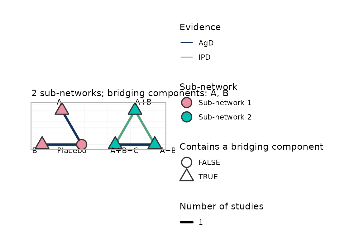

Step 1: connect with component NMA

cnma_bridge() fits the additive component model and reconstructs the relative effects across the gap.

br <- cnma_bridge(net)
component_effects(br)
#>   component  estimate        se     lower    upper statistic      pval
#> 1         A 0.5000000 1.1922140 -1.836697 2.836697 0.4193878 0.6749328
#> 2         B 0.4000000 1.1922140 -1.936697 2.736697 0.3355102 0.7372402
#> 3         C 0.7170248 0.9734562 -1.190914 2.624964 0.7365763 0.4613800
#> 4         D 0.3250136 0.9728622 -1.581761 2.231788 0.3340798 0.7383193

Step 2: adjust for effect modifiers

Components C and D come from the IPD studies, whose effect modifier x1 is imbalanced relative to the target population (x1 = 0). Anchored STC fits an outcome regression with treatment-by-x1 interactions and reads off the treatment effect at the target.

fit_stc <- cstc(net, target = c(x1 = 0), effect_modifiers = "x1")
component_effects(fit_stc)
#>   component  estimate        se        lower     upper statistic        pval
#> 1         A 0.5000000 0.2563324 -0.002402322 1.0024023  1.950592 0.051105590
#> 2         B 0.4000000 0.2563324 -0.102402322 0.9024023  1.560474 0.118647988
#> 3         C 0.4896667 0.2406290  0.018042458 0.9612910  2.034944 0.041856471
#> 4         D 0.6408956 0.2317142  0.186744196 1.0950470  2.765889 0.005676788

Anchored MAIC instead reweights each IPD study to the target population.

fit_maic <- cmaic(net, target = c(x1 = 0), effect_modifiers = "x1",
                  n_boot = 100, seed = 1)
effective_sample_size(fit_maic)
#>       S3       S4 
#> 207.4202 358.1461

Population adjustment moves the C and D effects relative to the unadjusted (naive) bridge, while the placebo-anchored components A and B are unchanged:

data.frame(
  component = component_effects(br)$component,
  naive     = round(component_effects(br)$estimate, 3),
  cSTC      = round(component_effects(fit_stc)$estimate, 3),
  cMAIC     = round(component_effects(fit_maic)$estimate, 3)
)
#>   component naive  cSTC cMAIC
#> 1         A 0.500 0.500 0.500
#> 2         B 0.400 0.400 0.400
#> 3         C 0.717 0.490 0.697
#> 4         D 0.325 0.641 0.772

Reporting

relative_effects(fit_stc)
#> Relative effects (OR, back-transformed)
#>  treatment comparator estimate    se lower  upper     z     p
#>          A    Placebo    1.649 0.256 0.998  2.725 1.951 0.051
#>        A+B    Placebo    2.460 0.363 1.209  5.005 2.483 0.013
#>      A+B+C    Placebo    4.014 0.435 1.711  9.416 3.194 0.001
#>      A+B+D    Placebo    4.669 0.430 2.009 10.850 3.582 0.000
#>          B    Placebo    1.492 0.256 0.903  2.466 1.560 0.119
additivity_test(fit_stc)
#> Additive component model: fit statistics
#>   Total lack of fit (Q.additive): Q = 2.669, df = 1, p = 0.102
#>   Additivity restrictions (Q.diff): not available; no standard NMA
#>     is estimable on a disconnected network.
#>   Note: neither statistic tests whether component effects are constant
#>   ACROSS sub-networks, which is the assumption that bridges the gap.
#>   That assumption is untestable from the data and must be justified
#>   clinically.

forest(fit_stc)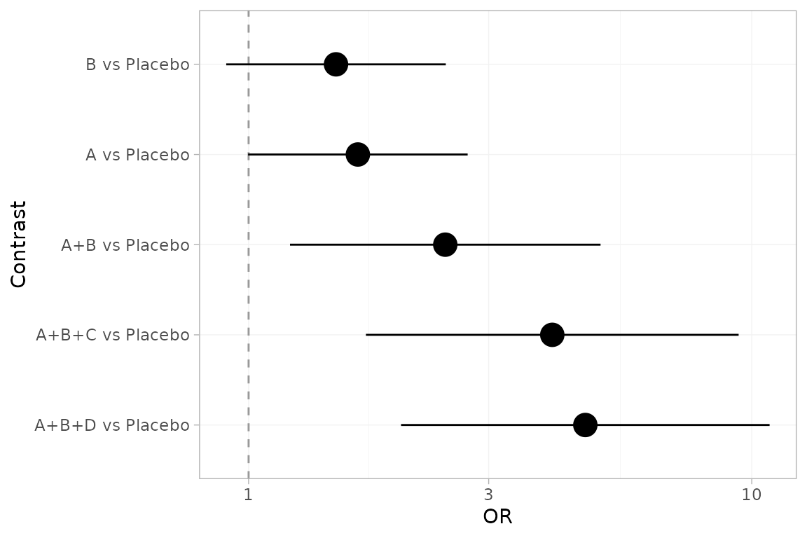

Where next

• vignette("cpaic-methods") covers the statistical framework in depth.
• The full mathematical foundations and a validation study are provided with the development sources.