Summarizing transparency across a corpus • rtransparency

The detector functions (rt_all_pmc(), rt_data_code_pmc()) describe one article at a time. Most studies of research transparency instead ask corpus-level questions: across thousands of articles, how often is each practice present? Is it improving over time? Does it differ by journal or article type?

This vignette shows how to go from per-article detector output to that kind of summary, using rt_summary(), rt_score() and rt_plot().

From one article to many

Running a detector on a single article returns a one-row table of indicators:

library(rtransparency)
#> rtransparency 1.1.0: identify indicators of transparency (conflicts of interest, funding,
#> protocol registration, novelty, replication, data and code sharing, AI-use disclosure,
#> open-access licensing and reporting-guideline use) in biomedical articles. GitHub: https://github.com/choxos/rtransparency | vignette("rtransparency")

xml <- system.file(
  "extdata", "PMID32171256-PMC7071725.xml", package = "rtransparency"
)
one <- rt_all_pmc(xml, remove_ns = TRUE)
one[, c("pmid", "is_coi_pred", "is_fund_pred", "is_register_pred")]
#> # A tibble: 1 × 4
#>   pmid     is_coi_pred is_fund_pred is_register_pred
#>   <chr>    <lgl>       <lgl>        <lgl>           
#> 1 32171256 TRUE        FALSE        FALSE

To study a corpus you run a detector over many files and stack the rows; purrr::map_dfr(files, rt_all_pmc, remove_ns = TRUE) returns all ten indicators per article in one pass. The result is one row per article with the indicator columns is_coi_pred, is_fund_pred, is_register_pred, is_open_data, is_open_code, is_novelty_pred, is_replication_pred, is_ai_pred, is_open_access and is_reporting_pred. is_ai_pred is NA for articles published before 2023, and rt_summary() drops those NAs, so the AI-disclosure prevalence is computed only over the articles where the indicator applies. is_open_access and is_reporting_pred are summarized by rt_summary() too, but are not part of the five openness practices counted by rt_score().

This package ships a small simulated table of that shape, rt_demo, so the rest of the vignette runs without downloading anything:

data(rt_demo)
head(rt_demo)
#> # A tibble: 6 × 11
#>   pmid      year type     is_coi_pred is_fund_pred is_register_pred is_open_data
#>   <chr>    <int> <chr>    <lgl>       <lgl>        <lgl>            <lgl>       
#> 1 28143943  2011 review-… FALSE       TRUE         TRUE             FALSE       
#> 2 31314758  2014 systema… FALSE       TRUE         TRUE             FALSE       
#> 3 30397608  2022 systema… TRUE        TRUE         FALSE            TRUE        
#> 4 37703615  2026 researc… TRUE        TRUE         TRUE             TRUE        
#> 5 26030375  2022 researc… TRUE        TRUE         FALSE            FALSE       
#> 6 21738034  2018 researc… TRUE        TRUE         FALSE            FALSE       
#> # ℹ 4 more variables: is_open_code <lgl>, is_novelty_pred <lgl>,
#> #   is_replication_pred <lgl>, is_ai_pred <lgl>

Prevalence of each indicator

rt_summary() reports, for each indicator, how many articles were assessed, how many were positive, the apparent prevalence and its 95% confidence interval:

s <- rt_summary(rt_demo)
knitr::kable(
  s[, c("label", "n_articles", "n_detected", "percent", "conf_low", "conf_high")],
  digits = 1,
  col.names = c("Indicator", "Assessed", "Detected", "%", "CI low", "CI high")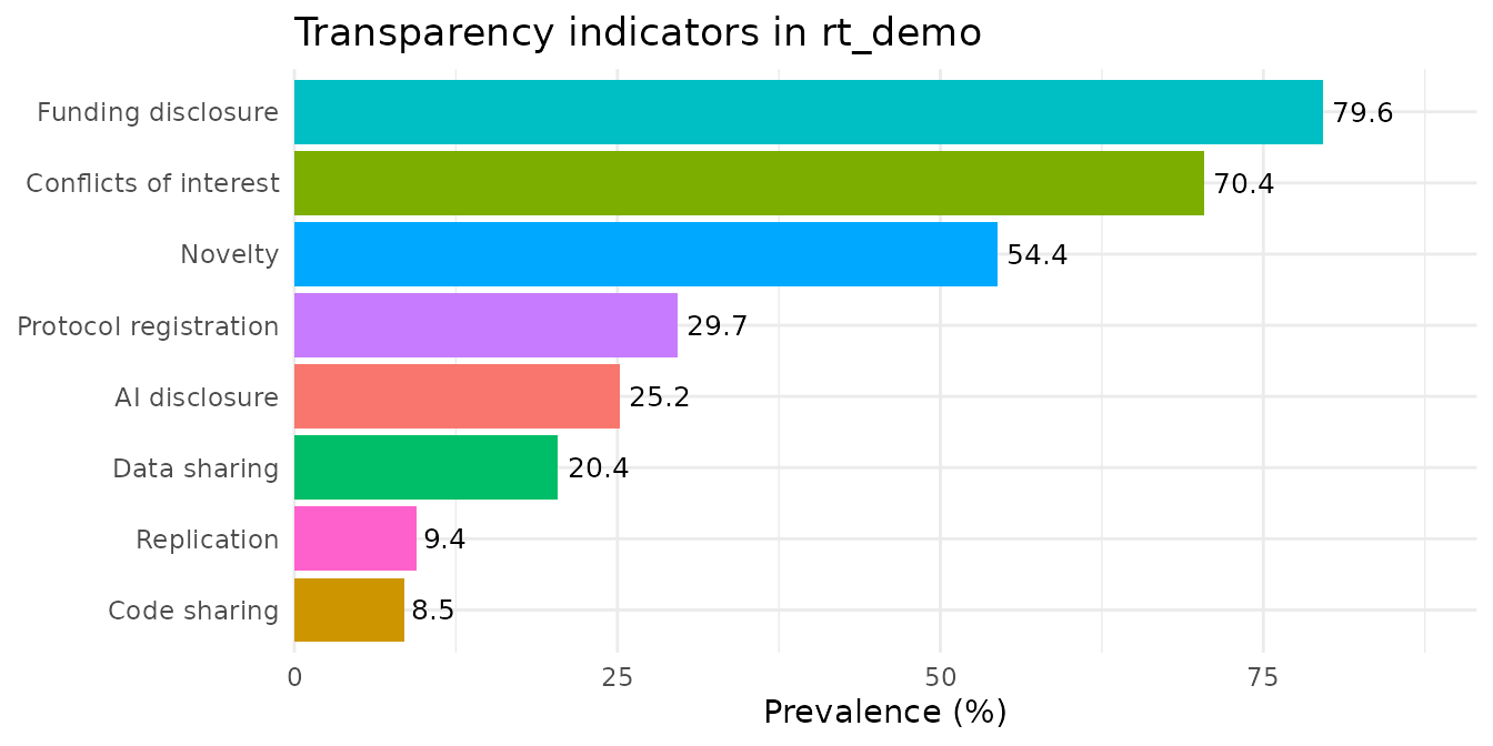
)

Indicator	Assessed	Detected	%	CI low	CI high
Conflicts of interest	1200	845	70.4	67.8	72.9
Funding disclosure	1200	955	79.6	77.2	81.8
Protocol registration	1200	356	29.7	27.2	32.3
Data sharing	1200	245	20.4	18.2	22.8
Code sharing	1200	102	8.5	7.1	10.2
Novelty	1200	653	54.4	51.6	57.2
Replication	1200	113	9.4	7.9	11.2
AI disclosure	282	71	25.2	20.5	30.6

Correcting for detector error

A text-mining detector is not perfect, so the observed prevalence is a biased estimate of the true prevalence. rt_summary() corrects for this using each detector’s sensitivity and specificity estimates (the Rogan-Gladen estimator). The correction is on by default and adds adj_percent, adj_low and adj_high:

knitr::kable(
  s[, c("label", "percent", "adj_percent", "adj_low", "adj_high")],
  digits = 1,
  col.names = c("Indicator", "Apparent %", "Corrected %", "CI low", "CI high")
)

Indicator	Apparent %	Corrected %	CI low	CI high
Conflicts of interest	70.4	70.8	68.2	73.4
Funding disclosure	79.6	79.4	77.0	81.7
Protocol registration	29.7	30.8	28.2	33.6
Data sharing	20.4	25.7	22.8	28.9
Code sharing	8.5	9.1	7.5	11.1
Novelty	54.4	62.8	59.2	66.3
Replication	9.4	8.7	7.0	10.6
AI disclosure	25.2	NA	NA	NA

The accuracy values come from rt_accuracy:

rt_accuracy
#> # A tibble: 8 × 5
#>   variable            label                 sensitivity specificity source      
#>   <chr>               <chr>                       <dbl>       <dbl> <chr>       
#> 1 is_coi_pred         Conflicts of interest       0.992       0.995 Serghiou et…
#> 2 is_fund_pred        Funding disclosure          0.997       0.981 Serghiou et…
#> 3 is_register_pred    Protocol registration       0.955       0.997 Serghiou et…
#> 4 is_open_data        Data sharing                0.765       0.99  rtransparen…
#> 5 is_open_code        Code sharing                0.881       0.995 rtransparen…
#> 6 is_novelty_pred     Novelty                     0.838       0.952 rtransparen…
#> 7 is_replication_pred Replication                 0.928       0.985 rtransparen…
#> 8 is_reporting_pred   Reporting guideline         0.938       0.99  rtransparen…

AI-use disclosure has no bundled accuracy estimate here, so its corrected value is NA. Novelty’s estimate comes from a hand-labeled gold set (inst/benchmark/results_novelty_replication.md); the data/code values are reproducible benchmark estimates for the native detector, not untouched external-validation estimates. Replication’s correction is approximate: its sensitivity comes from a replication-enriched sample and its specificity from the representative 2023 sample, so it does not rest on the single-design validation of conflicts of interest, funding or registration, and the Rogan-Gladen interval does not propagate uncertainty in these estimates. To use your own validation (or the published oddpub values for data and code), pass any table with variable, sensitivity and specificity columns:

my_acc <- rt_accuracy
my_acc$sensitivity[my_acc$variable == "is_open_data"] <- 0.758
rt_summary(rt_demo, indicators = "is_open_data", accuracy = my_acc)[,
  c("label", "percent", "adj_percent")]
#> # A tibble: 1 × 3
#>   label        percent adj_percent
#>   <chr>          <dbl>       <dbl>
#> 1 Data sharing    20.4        26.0

How many practices per article

rt_score() adds a per-article count of the openness practices met (conflicts of interest, funding, registration, data and code). Tabulating it shows how many articles meet zero, one, two … of the five practices:

scored <- rt_score(rt_demo)
knitr::kable(
  as.data.frame(table(`Practices met` = scored$n_indicators)),
  col.names = c("Practices met", "Articles")
)

Practices met	Articles
0	52
1	288
2	467
3	305
4	74
5	14

Subgroups

Pass by to summarize within a grouping column, such as article type:

by_type <- rt_summary(rt_demo, by = "type", adjust = FALSE)
knitr::kable(
  by_type[by_type$indicator == "is_open_data",
          c("type", "label", "n_articles", "percent")],
  digits = 1,
  col.names = c("Type", "Indicator", "Assessed", "%")
)

Type	Indicator	Assessed	%
review-article	Data sharing	241	19.5
systematic-review	Data sharing	132	23.5
research-article	Data sharing	827	20.2

Plots

rt_plot() returns a ggplot, so it composes with the usual ggplot2 layers. The default is a prevalence bar chart:

library(ggplot2)
rt_plot(rt_demo) + ggtitle("Transparency indicators in rt_demo")

Bar chart of the prevalence of each transparency indicator

Use type = "trend" with a year column to see prevalence over time:

rt_plot(rt_demo, type = "trend", year = "year")
#> Warning: Removed 13 rows containing missing values or values outside the scale range
#> (`geom_line()`).
#> Warning: Removed 13 rows containing missing values or values outside the scale range
#> (`geom_point()`).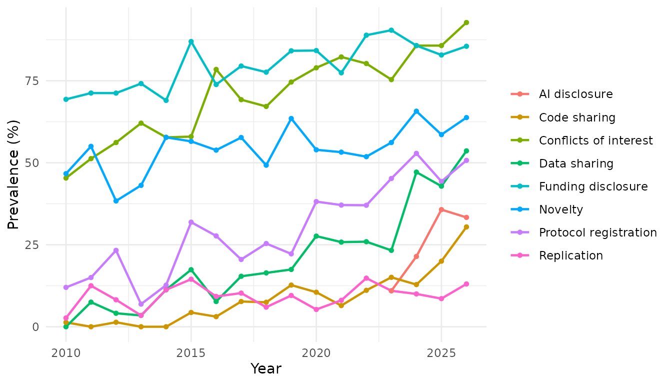

Line chart of each transparency indicator's prevalence by year

The AI-disclosure line begins only in 2023, because the indicator is NA before then; the rising data-sharing and AI lines illustrate the kind of trend these summaries are meant to surface. Restrict a plot to particular indicators with indicators =, for example to follow AI-use disclosure on its own:

rt_plot(rt_demo, type = "trend", year = "year", indicators = "is_ai_pred") +
  ggtitle("Disclosure of generative-AI use, 2023 onward")
#> Warning: Removed 13 rows containing missing values or values outside the scale range
#> (`geom_line()`).
#> Warning: Removed 13 rows containing missing values or values outside the scale range
#> (`geom_point()`).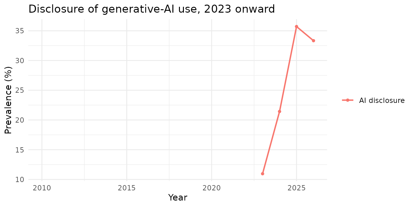

Line chart of AI-use disclosure prevalence by year from 2023

Set adjusted = TRUE in either plot to show the error-corrected prevalence instead of the apparent prevalence.

Putting it together

A typical analysis is therefore: run a detector over your corpus, stack the rows, then

results <- purrr::map_dfr(xml_files, rt_all_pmc, remove_ns = TRUE)
rt_summary(results)                       # prevalence + corrected prevalence
rt_score(results)                         # per-article practice count
rt_plot(results, type = "trend", year = "year")

For the per-indicator detection methodology, see vignette("rtransparency").