Illustrating and interpreting a FAIR assessment • rfair

This vignette shows how to read the output of an assessment: the scorecard plot, the score tables, the maturity levels, and the reuse/access context that rfair adds on top of the F-UJI metrics. For how the scores are computed see vignette("methodology"); for a quick tour see vignette("rfair").

So the vignette renders offline and deterministically, it uses the bundled example assessment fair_example (a real assessment of a Zenodo deposit, ). You produce your own the same way:

# (needs network) assess any DOI / PID / URL:
x <- assess_fair("https://doi.org/10.5281/zenodo.8347772")

data(fair_example)
x <- fair_example
x
#> <fair_assessment> https://doi.org/10.5281/zenodo.8347772
#>   resolved: https://zenodo.org/records/8347772
#>   metrics: v0.8 (17 metrics)
#> 
#>   FAIR     earned  percent  maturity
#>   F           7/7   100.0%         3
#>   A           7/7   100.0%         3
#>   I           4/6    66.7%         2
#>   R           5/6    83.3%         2
#>   FAIR      23/26    88.5%       2.5
#> 
#>   reuse:    open (software, permissive); custom/unknown

The printed summary is the fastest read: an earned/total and percentage per FAIR category, the overall score, and any reuse/access/identifier flags.

1. The scorecard plot

plot() turns the assessment into a one-glance scorecard. Each bar is a FAIR category filled to its score, labeled with earned/total and its maturity level (the colored word on the right). The dark bar at the top is the overall FAIR score.

plot(x)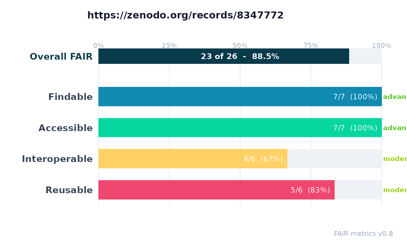

FAIR scorecard: horizontal bars for Findable, Accessible, Interoperable and Reusable, plus an overall FAIR bar.

To see which of the 17 metrics drive each category, plot the per-metric breakdown. Bars are grouped and colored by category (F/A/I/R) and labeled with the metric identifier and its earned/total.

plot(x, type = "metric")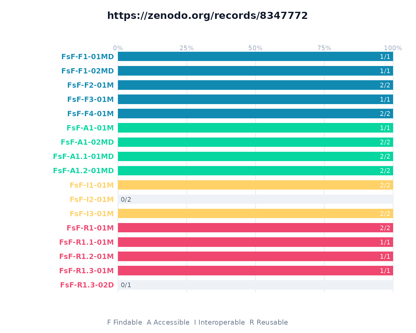

Per-metric FAIR breakdown: one horizontal bar per metric, grouped by category.

For a compact overview that shows both levels at once, type = "sunburst" draws a concentric ring chart: the inner ring is the four FAIR categories and the outer ring is the individual metrics, each filled in proportion to its score, with the overall FAIR percentage in the center. This is the same summary the web app shows.

plot(x, type = "sunburst")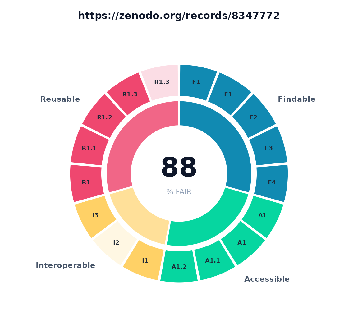

Concentric FAIR sunburst: inner ring of F/A/I/R categories, outer ring of individual metrics, overall percentage in the center.

2. Score tables

summary() returns the per-category table behind the scorecard (handy for reports and further computation):

summary(x)
#>   category earned total percent maturity
#> 1        F      7     7  100.00      3.0
#> 2        A      7     7  100.00      3.0
#> 3        I      4     6   66.67      2.0
#> 4        R      5     6   83.33      2.0
#> 5     FAIR     23    26   88.46      2.5

as.data.frame() gives one row per metric, with its principle, category, score, maturity, and pass/fail status:

df <- as.data.frame(x)
head(df, 8)
#>   metric_identifier principle category
#> 1       FsF-F1-01MD        F1        F
#> 2       FsF-F1-02MD        F1        F
#> 3        FsF-F2-01M        F2        F
#> 4        FsF-F3-01M        F3        F
#> 5        FsF-F4-01M        F4        F
#> 6        FsF-A1-01M        A1        A
#> 7       FsF-A1-02MD        A1        A
#> 8     FsF-A1.1-01MD      A1.1        A
#>                                                                                                                                                     metric_name
#> 1                                                                                                  Metadata and data are assigned a globally unique identifier.
#> 2                                                                                                       Metadata and data are assigned a persistent identifier.
#> 3 Metadata includes descriptive core elements (creator, title, data identifier, publisher, publication date, summary and keywords) to support data findability.
#> 4                                                                                                    Metadata includes the identifier of the data it describes.
#> 5                                                                     Metadata is offered in such a way that it can be registered or indexed by search engines.
#> 6                                                                                             Metadata contains access level and access conditions of the data.
#> 7                                                                                                         Metadata and data are retrievable by their identifier
#> 8                                                                                    A standardized communication protocol is used to access metadata and data.
#>   earned total percent maturity status
#> 1      1     1     100        3   pass
#> 2      1     1     100        3   pass
#> 3      2     2     100        3   pass
#> 4      1     1     100        3   pass
#> 5      2     2     100        3   pass
#> 6      1     1     100        3   pass
#> 7      2     2     100        3   pass
#> 8      2     2     100        3   pass

Because it is a plain data frame you can slice it however you like, for example the metrics that did not earn full marks:

df[df$earned < df$total, c("metric_identifier", "metric_name", "earned", "total")]
#>    metric_identifier
#> 11        FsF-I2-01M
#> 17      FsF-R1.3-02D
#>                                                                         metric_name
#> 11                                      Metadata uses registered semantic resources
#> 17 Data is available in a file format recommended by the target research community.
#>    earned total
#> 11      0     2
#> 17      0     1

3. How to read the numbers

Score (earned/total). Each metric is worth a fixed number of points; the category score is the sum of earned over total across its metrics, and the overall FAIR score is the sum across all 17 metrics.
Percent. earned / total * 100, shown on each bar.
Maturity (FAIR level). A CMMI level from 0 to 3 (incomplete, initial, moderate, advanced) summarizing how far up the testing ladder a metric reached. A metric can earn points yet still sit at a low maturity if only its easiest test passed. Maturity is the colored tag on the category scorecard.
A low score is a finding, not a verdict. A restricted-access or unlicensed object can be perfectly legitimate; the score tells you what a machine could and could not verify from the metadata.

4. The context rfair adds beyond the score

A single FAIR percentage hides why an object is or is not reusable. rfair surfaces that separately (see vignette("beyond-fuji")); the same information is in the assessment object and worth showing alongside the scorecard.

License reusability (not merely presence): a license can be detected yet not actually permit reuse.

x$reuse$licenses[[1]][c("license", "category", "rdp_category")]
#> $license
#> [1] "https://opensource.org/licenses/MIT"
#> 
#> $category
#> [1] "open (software, permissive)"
#> 
#> $rdp_category
#> [1] "permissive"

Access level and sensitivity flags (a restricted object is not a FAIR failure, but you should know):

x$access[c("access", "controlled_access", "sensitive")]
#> $access
#> [1] "public"
#> 
#> $controlled_access
#> [1] FALSE
#> 
#> $sensitive
#> [1] FALSE

Identifier hygiene (does the persistent identifier resolve cleanly, no obvious problems):

x$identifier_hygiene[c("scheme", "is_persistent", "hygiene_ok")]
#> $scheme
#> [1] "doi"
#> 
#> $is_persistent
#> [1] TRUE
#> 
#> $hygiene_ok
#> [1] TRUE

5. Exporting the illustration

The assessment serializes for downstream tools. as_fuji_json() emits a payload matching the upstream F-UJI FAIRResults schema:

js <- as_fuji_json(x)
substr(js, 1, 220)
#> {
#>   "test_id": "4114fa229002ed3433f77ebd3857888da20b07c6",
#>   "request": {
#>     "object_identifier": "https://doi.org/10.5281/zenodo.8347772",
#>     "metric_version": "0.8",
#>     "use_datacite": true,
#>     "test_debug": false
#>

as_rdf() emits a machine-readable rating (W3C DQV plus a schema.org Rating as JSON-LD), suitable for embedding in a landing page:

rdf <- as_rdf(x)
substr(rdf, 1, 220)
#> [1] "{\n  \"@context\": {\n    \"dcat\": \"http://www.w3.org/ns/dcat#\",\n    \"dc\": \"http://purl.org/dc/terms/\",\n    \"schema\": \"http://schema.org/\",\n    \"dqv\": \"http://www.w3.org/ns/dqv#\",\n    \"prov\": \"http://www.w3.org/ns/prov#\",\n   "

Summary

plot(x) and plot(x, type = "metric") are the quickest way to see an assessment.
summary(x) and as.data.frame(x) give the numbers as tidy tables.
Read score, percent, and maturity together; treat low scores as questions, not verdicts.
The reuse, access, and identifier-hygiene elements explain the why behind the number.