
responder_analysis() and responder_from_effect() return a
responder_result: a data frame with one row per method (so $, [ and
column access work as usual) that also keeps the analysis settings and the
per-study statistics. print() shows a formatted table with the number
needed to treat; summary() adds the settings, heterogeneity statistics and
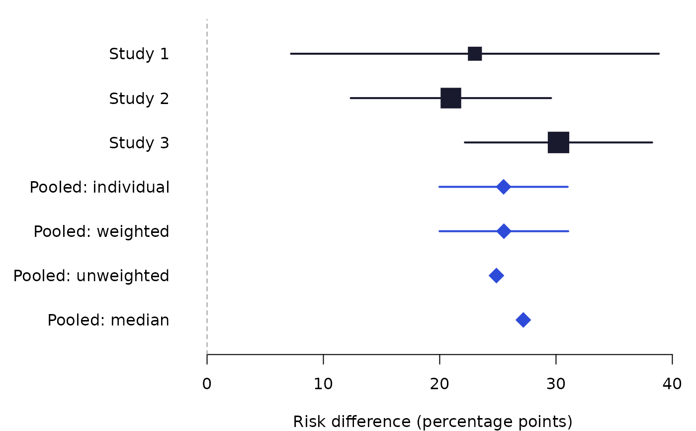
per-study weights; plot() draws a forest plot of the per-study and pooled
risk differences; as.data.frame() returns the plain numeric table.
Usage
# S3 method for class 'responder_result'
print(x, digits = 1, ...)

# S3 method for class 'responder_result'
x[i, j, drop = FALSE]

# S3 method for class 'responder_result'
summary(object, ...)

# S3 method for class 'summary.responder_result'
print(x, digits = 1, ...)

# S3 method for class 'responder_result'
as.data.frame(x, row.names = NULL, optional = FALSE, ...)

# S3 method for class 'responder_result'
plot(x, ...)
Arguments
- x, object
A
responder_result.- digits
Decimal places for percentages.
- ...
Unused (for
plot(), passed tographics::plot()).- i, j
Row and column indices.
- drop
Passed to the data-frame method.
- row.names, optional
Passed to
as.data.frame().
Value
print() and plot() return x invisibly; summary() returns a
summary.responder_result list; as.data.frame() returns a data frame.
Examples
res <- responder_analysis(sample_responder_data, mid = 1)
res
#> Responder analysis (respondeR)
#> MID = 1 (a higher change is a response); k = 3 studies; fixed
#> effects; delta per-study variance
#> Percentages; 95% confidence intervals.
#>
#> Method PE PC RD RR
#> Individual - - 25.5 (20.0 to 31.0) 2.15 (1.79 to 2.58)
#> Weighted mean 47.6 22.1 25.5 (20.0 to 31.1) 2.16 (1.80 to 2.59)
#> Unweighted mean 47.7 22.8 24.9 2.09
#> Median 48.7 21.5 27.2 2.26
#> OR NNT
#> 3.20 (2.45 to 4.18) NNTB 3.9 (3.2 to 5.0)
#> 3.21 (2.46 to 4.19) NNTB 3.9 (3.2 to 5.0)
#> 3.09 NNTB 4.0
#> 3.46 NNTB 3.7
#>
#> Use as.data.frame() for every column, summary() for details, plot() for a forest plot.
summary(res)
#> Responder analysis (respondeR): summary
#>
#> mid 1
#> direction higher
#> se_method delta
#> pooling fixed
#> control matched
#> tau_method DL
#> ci_method wald
#> rd_weights sample_size
#> dist normal
#> mid_sd 0
#> ci_type wald
#> conf_level 0.95
#> k 3
#> median p_c 22.6%
#>
#> Method PE PC RD RR
#> Individual - - 25.5 (20.0 to 31.0) 2.15 (1.79 to 2.58)
#> Weighted mean 47.6 22.1 25.5 (20.0 to 31.1) 2.16 (1.80 to 2.59)
#> Unweighted mean 47.7 22.8 24.9 2.09
#> Median 48.7 21.5 27.2 2.26
#> OR NNT
#> 3.20 (2.45 to 4.18) NNTB 3.9 (3.2 to 5.0)
#> 3.21 (2.46 to 4.19) NNTB 3.9 (3.2 to 5.0)
#> 3.09 NNTB 4.0
#> 3.46 NNTB 3.7
#>
#> Heterogeneity (scale pooled: RD for individual, g for smd):
#> method tau2 i2 q q_p pi_lb pi_ub
#> individual 0.000631 0.193 2.48 0.29 NA NA
#>
#> Per-study responder statistics (individual method):
#> study p_e p_c rd weight
#> Study 1 48.7 25.6 23.0 12.8%
#> Study 2 43.6 22.6 21.0 41.2%
#> Study 3 50.7 20.5 30.2 46.1%
plot(res)
 head(as.data.frame(res), 2)
#> method pooling k p_e p_c rd rd_lb rd_ub
#> 1 individual fixed 3 NA NA 0.2548985 0.1997582 0.3100388
#> 2 weighted fixed 3 0.4757294 0.2205372 0.2551921 0.1998579 0.3105264
#> rr rr_lb rr_ub or or_lb or_ub nnt nnt_lb
#> 1 2.148360 1.787463 2.582123 3.197922 2.447367 4.178656 3.923130 3.225403
#> 2 2.157138 1.795354 2.591827 3.207140 2.455182 4.189402 3.918616 3.220338
#> nnt_ub var_rd tau2 i2 q q_p pi_lb pi_ub
#> 1 5.006053 0.0007914838 0.0006313298 0.1925461 2.476921 0.28983 NA NA
#> 2 5.003555 0.0007970618 NA NA NA NA NA NA