What is the Quality of Care Index (QCI)?
The Quality of Care Index (QCI) is a composite metric derived from Global Burden of Disease (GBD) study data. It uses Principal Component Analysis (PCA) on four epidemiological ratios to produce a single score (0-100) for each country, year, and sex combination. Higher scores indicate better quality of care.
The four component ratios are:
- MIR: Mortality-to-Incidence Ratio (Deaths / Incidence)
- YLLtoYLD: Years of Life Lost to Years Lived with Disability ratio
- DALtoPER: DALY-to-Prevalence Ratio
- PERtoINC: Prevalence-to-Incidence Ratio
Quick Start
Loading Sample Data
The package includes sample GBD data for demonstration:
data(sample_gbd)
head(sample_gbd[, c("location_name", "measure_name", "metric_name", "year", "val")])
#>   location_name                       measure_name metric_name year      val
#> 1         Japan YLDs (Years Lived with Disability)        Rate 1990 2.674029
#> 2         Japan YLDs (Years Lived with Disability)        Rate 1990 2.779096
#> 3         Japan YLDs (Years Lived with Disability)        Rate 1990 2.723352
#> 4         China YLDs (Years Lived with Disability)        Rate 1990 3.612208
#> 5         China YLDs (Years Lived with Disability)        Rate 1990 4.225407
#> 6         China YLDs (Years Lived with Disability)        Rate 1990 3.910120
Running the Pipeline
The qci_pipeline() function runs the entire analysis in
one call:
result <- qci_pipeline(sample_gbd, verbose = FALSE)
#> ✔ Cleaned data: 9 locations, 3 years.
#> ℹ PCA done for "Both / Age-standardized": 74.1% variance explained (n=27).
#> ℹ PCA done for "Female / Age-standardized": 75.7% variance explained (n=27).
#> ℹ PCA done for "Male / Age-standardized": 73.2% variance explained (n=27).
The result is a list with three elements:
names(result)
#> [1] "wide"        "long"        "pca_details"
Examining Results
Wide format - one row per location/year/sex:
result$wide[, .(location_name, year, sex_name, qci_score)] |>
  head(10)
#> Key: <location_name, year, sex_name>
#>     location_name  year sex_name qci_score
#>            <char> <int>   <char>     <num>
#>  1:     Australia  1990     Both  99.96851
#>  2:     Australia  1990   Female  99.96648
#>  3:     Australia  1990     Male  99.94012
#>  4:     Australia  2005     Both 100.00000
#>  5:     Australia  2005   Female  99.91433
#>  6:     Australia  2005     Male  99.97438
#>  7:     Australia  2019     Both  99.98164
#>  8:     Australia  2019   Female 100.00000
#>  9:     Australia  2019     Male 100.00000
#> 10:        Brazil  1990     Both   0.00000
PCA details - variance explained by the first principal component:
result$pca_details
#>   sex_name         age_name variance_explained_pc1 eigenvalue_pc1
#> 1     Both Age-standardized               74.05598       2.962239
#> 2   Female Age-standardized               75.66964       3.026785
#> 3     Male Age-standardized               73.20481       2.928192
#>   n_observations
#> 1             27
#> 2             27
#> 3             27
Gender Disparity Ratio
Compute the GDR (Female QCI / Male QCI):
gdr <- qci_gdr(result$wide)
head(gdr[, .(location_name, year, qci_female, qci_male, gdr, gdr_category)])
#>    location_name  year qci_female  qci_male       gdr gdr_category
#>           <char> <int>      <num>     <num>     <num>       <char>
#> 1:         China  1990   19.01955  2.425957 7.8400189         high
#> 2:         China  2005   53.22120 55.349268 0.9615519        equal
#> 3:         China  2019   83.53537 92.311271 0.9049315          low
#> 4:         Japan  1990   98.90032 98.579658 1.0032528        equal
#> 5:         Japan  2005   98.57262 99.512890 0.9905512        equal
#> 6:         Japan  2019   94.94150 99.428526 0.9548718        equal
Visualization
Trend plot:
plot_qci_trend(result$wide,
               locations = unique(result$wide$location_name)[1:3])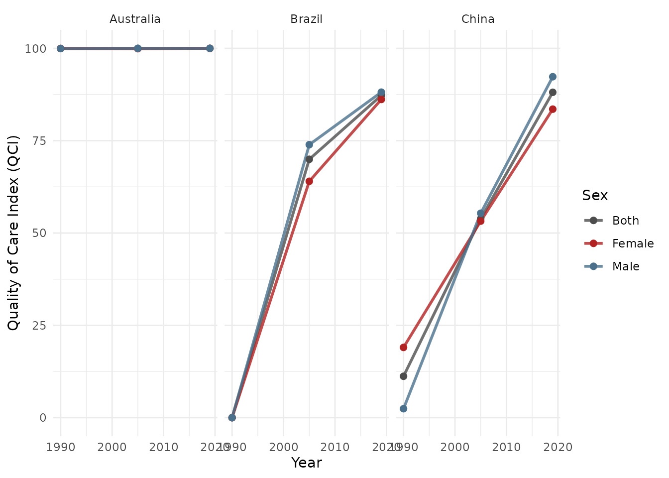
Distribution plot:
plot_qci_distribution(result$wide, years = c(1990, 2019))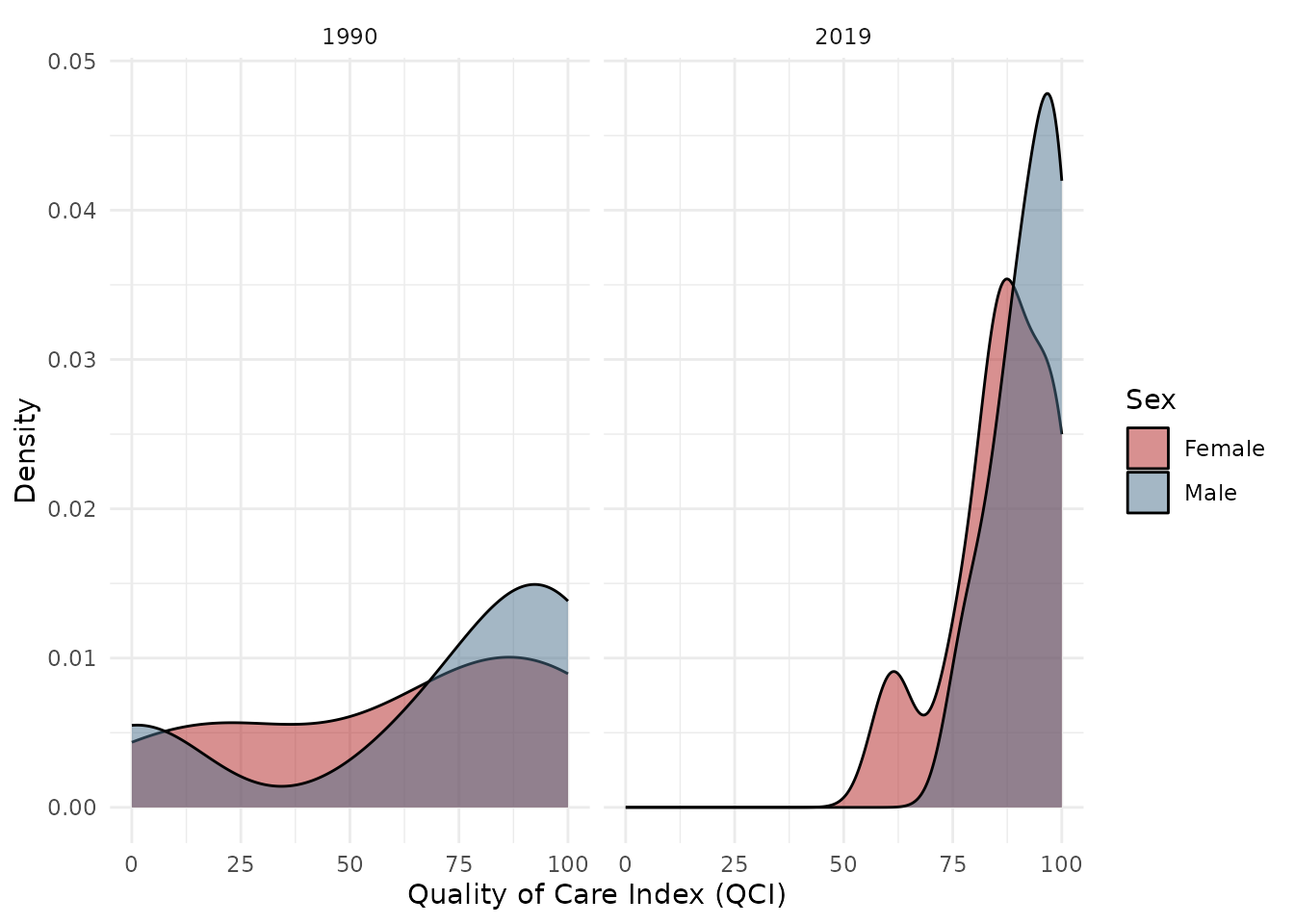
Using Your Own GBD Data
- Export data from the GBD Results Tool
- Ensure you include all 6 measures: Deaths, Incidence, Prevalence, DALYs, YLLs, YLDs
- Include both Rate and Number metrics
- Load and process:
# Single file
result <- qci_pipeline("path/to/gbd_export.csv")

# Multiple files (merged automatically)
result <- qci_pipeline(c("file1.csv", "file2.csv", "file3.csv"))
Step-by-Step Analysis
For more control, use individual functions:
# 1. Load
gbd <- qci_load("path/to/gbd_data.csv")

# 2. Clean and reshape
cleaned <- qci_clean(gbd)

# 3. Compute ratios
with_ratios <- qci_ratios(cleaned$wide_number)

# 4. Run PCA
pca_result <- qci_pca(with_ratios)

# 5. Gender disparity
gdr <- qci_gdr(pca_result$data)

# 6. Export
qci_export_csv(pca_result$data, "qci_results.csv")